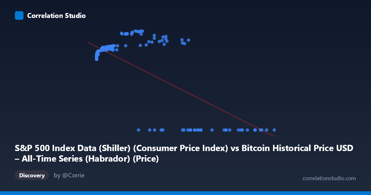
S&P 500 Index Data (Shiller) (Consumer Price Index) vs Bitcoin Historical Price USD – All-Time Series (Habrador) (Price)
- Pearson correlation (r)
- -0.7354
- Spearman correlation
- 0.1008
- p-value
- 0
- Sample size (n)
- 189
- 95% confidence interval
- -0.7947 to -0.6622
- Granger causality
- Y → X
- Granger optimal lag
- 4
- Time coverage
- 2010-08-01 to 2026-04-01
- Recomputed on refreshed data
- 2026-10-11 (r was -0.7354)
AI analysis
Analysis of Bitcoin Price vs. CPI Relationship
1. What the Visualization Reveals
The scatterplot shows a peculiar bifurcated pattern rather than a clean linear relationship. At low X-values (roughly 0–60,000), Y values cluster tightly in the 218–306 range, showing a mild positive relationship as X increases from near-zero. However, at higher X-values (above ~27,000), a large cluster of points collapses to Y=0, creating a stark discontinuity. This bimodal structure — a smooth curve for small X paired with a flat zero-line for larger X — is the dominant visual feature, and it strongly suggests two distinct regimes or a data-quality artifact rather than a single continuous relationship.
2. Strength, Direction, and Statistical Context
The reported r = -0.7354 (R² = 0.541) indicates a strong negative linear association, with 54% of Y's variance "explained" by X. The 95% CI [-0.7947, -0.6622] is fairly tight and excludes zero, and p ≈ 0 confirms this is not a chance finding in the sampled data. However, this negative slope is almost entirely an artifact of the zero-value cluster at high X — those points mechanically drag the correlation negative. The Granger causality results add an important temporal wrinkle: Y→X is significant (F=2.91, p=0.023) while X→Y is not (p=0.056), suggesting that historically, movements in the S&P/CPI series have some predictive power over Bitcoin price patterns, but not vice versa — though both p-values are marginal and the "4-period lag" designation warrants scrutiny given the mismatched, irregularly-sampled time series.
3. Notable Patterns and Outliers
The most striking feature is the hard floor at Y=0 for many high-X observations (e.g., X=27,983 → Y=0; X=118,670 → Y=0), sitting alongside genuine high-Y points at similarly large X values (X=44,354 → Y=287.5; X=56,973 → Y=278.8). This is inconsistent with a smooth functional relationship and looks like missing/null data encoded as zero rather than a true observation. Excluding the zero-cluster, the remaining data show a monotonic, decelerating (log-like) increase in Y with X — consistent with Bitcoin's price (X) growing across orders of magnitude while the paired index value (Y) rises then plateaus in the 230–306 range, typical of a bounded index against an exponentially-scaled asset price.
4. Confounding Factors and Caveats
Several serious caveats apply. First, the axis labels appear swapped or mismatched in the metadata (X is labeled "S&P 500... CPI" but contains Bitcoin-scale values into the hundreds of thousands; Y is labeled "Bitcoin Price" but ranges only 0–306) — this strongly suggests a data-pairing or column-mislabeling error. Second, the zero-value cluster likely represents missing/未recorded data rather than true zeros, which would artificially inflate the negative correlation. Third, pairing monthly Shiller data (dating to 1871) with Bitcoin's full price history (existing only since 2009) via nearest-date matching introduces asynchronous alignment noise. Finally, both series are highly non-stationary trending series, so classic Pearson correlation and Granger tests can produce spurious results without differencing or detrending.
5. Actionable Recommendations
Before drawing conclusions, verify the column mapping and investigate the zero-value points — determine whether these represent true data or placeholders for missing values, and consider excluding or imputing them. Re-run the analysis on log-transformed X (given Bitcoin's exponential price growth) and only for the overlapping true time period (2010–present) rather than the 2010–2026 label as stated, and difference both series to address non-stationarity before trusting Granger causality results. Segmenting the analysis into the two apparent regimes (Y0 vs Y=0) separately, and validating with a larger, cleanly matched sample, would clarify whether a genuine economic relationship exists or whether the current statistics are dominated by a data artifact.
X dataset: Bitcoin Historical Price USD – All-Time Series (Habrador)
Y dataset: S&P 500 Index Data (Shiller)
Part of experiment: Bitcoin - Bitcoin Historical Price USD – All-Time Series (Habrador) vs S&P 500 Index Data (Shiller)