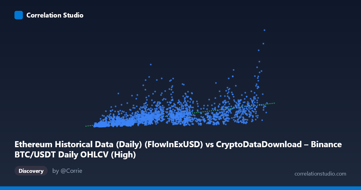
Ethereum Historical Data (Daily) (FlowInExUSD) vs CryptoDataDownload – Binance BTC/USDT Daily OHLCV (High)
- Pearson correlation (r)
- 0.6626
- Spearman correlation
- 0.8217
- p-value
- 0
- Sample size (n)
- 3191
- 95% confidence interval
- 0.6427 to 0.6816
- Granger causality
- Y → X
- Granger optimal lag
- 10
- Time coverage
- 2017-08-17 to 2026-05-20
AI analysis
Analysis: Cross-Chain Flow/Price Relationship (BTC vs ETH Metrics)
1. What the Visualization Reveals
The scatterplot shows a moderate positive relationship between an ETH-related flow metric (X) and BTC's daily high price (Y), with a distinctly heteroscedastic (funnel-shaped) pattern. As X increases, both the level and the spread of Y increase substantially — at low X values (~4,000–10,000), Y clusters tightly in the 50M–200M range, while at higher X values (~60,000–110,000), Y ranges wildly from ~300M to over 1.9B. This fanning pattern is a strong visual cue that the relationship is not simple linear proportionality but likely involves multiplicative or exponential scaling, consistent with the note that Spearman ρ exceeds Pearson r.
2. Strength, Direction, and Uncertainty
The correlation (r = 0.663, R² = 0.439) indicates a moderate-to-strong positive linear association, but only 43.9% of the variance in Y is explained by X — meaning more than half of the movement in BTC's high price is driven by factors outside this relationship. The tight confidence interval [0.643, 0.681] and p-value of ~0 confirm this correlation is highly statistically reliable and not a sampling artifact, despite the large unexplained variance. Critically, the Granger causality results reveal an asymmetric temporal structure: Y (BTC) Granger-causes X (ETH flow) at a 10-period lag (F=2.62, p=0.0036), while the reverse (X→Y) is not significant (p=0.134). This suggests BTC price movements precede and help predict ETH flow-in patterns — not the other way around — which is an important reframing: the correlation is not just contemporaneous co-movement but reflects BTC acting as a leading indicator for this ETH metric over ~10-day horizons.
3. Notable Patterns and Outliers
Several points stand out as high-leverage outliers: (64000, 1.79B), (56758, 1.36B), and (41100, 1.57B) show disproportionately high Y values relative to their X, sitting well above the regression line, while points like (101351, 633M) and (111308, 519M) show high X with comparatively modest Y — nearly inverting the general trend at the upper end. This suggests the relationship may saturate or even weaken at very high X values, or that these points correspond to distinct market regimes (e.g., different volatility periods, bull/bear phases, or exchange-specific liquidity events). The increasing variance with X (heteroscedasticity) also violates a key OLS assumption, meaning the linear regression's confidence intervals on predictions are likely understated at higher X ranges.
4. Confounding Factors and Caveats
This is a cross-asset comparison (ETH flow metrics vs. BTC price), so both series are likely driven by shared macro factors — overall crypto market sentiment, USD liquidity conditions, exchange-wide volume surges, or major news events — rather than a direct causal mechanism between ETH flows and BTC price. The ~9-year time span (2017–2026) also spans multiple distinct market regimes (2017 ICO boom, 2018 crash, 2020-21 bull run, 2022 collapse, subsequent recovery), and pooling all these regimes into one correlation risks Simpson's-paradox-style distortion — the "true" relationship may differ meaningfully across sub-periods. Additionally, since BTC's "High" column is a price level (non-stationary, trending series) and X is a flow-in volume (potentially more stationary), spurious correlation from shared trends/non-stationarity should be checked via cointegration testing before trusting Granger causality results.
5. Actionable Next Steps
1. Log-transform both variables given the heteroscedastic fan pattern and Spearman Pearson signal — a log-log or log-linear model will likely fit substantially better than the current linear specification. 2. Segment by market regime/year to test whether the r=0.66 correlation is stable or driven by specific bull-market periods; run rolling-window correlations. 3. Test for stationarity and cointegration (ADF/Johansen tests) before over-interpreting the Granger causality result, since trending price series can produce misleading Granger results. 4. Investigate the outlier cluster (the 41K–70K X-range points with Y 1.3B) — these may correspond to specific dates/events worth flagging separately. 5. Given BTC→X Granger causality, consider building a lagged predictive model (BTC high at t predicting ETH flow at t+10) as a more actionable trading/monitoring signal than the contemporaneous correlation.
X dataset: CryptoDataDownload – Binance BTC/USDT Daily OHLCV
Y dataset: Ethereum Historical Data (Daily)
Part of experiment: Bitcoin - CryptoDataDownload – Binance BTC/USDT Daily OHLCV vs Ethereum Historical Data (Daily)