S&P 500 Index Daily OHLCV (Date) (mavg) vs Cboe U.S. Equities Historical Market Volume Data 2015 (Tape B Trade Count)
- Pearson correlation (r)
- -0.4283
- Spearman correlation
- -0.4847
- p-value
- 0
- Sample size (n)
- 222
- 95% confidence interval
- -0.5301 to -0.3144
- Granger causality
- None
- Granger optimal lag
- 1
AI analysis
Scatterplot Analysis: S&P 500 Moving Average vs. Cboe Tape B Trade Count (2015)
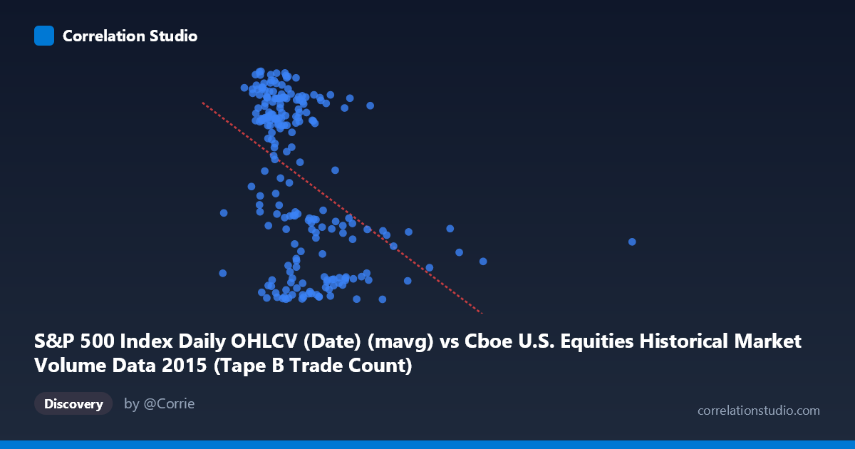
Relationship Overview The scatterplot reveals a negative relationship between the S&P 500 Index daily moving average (X) and the Cboe U.S. Equities Tape B trade count (Y), meaning that as the index's moving average rises, Tape B trade counts tend to decline. The linear regression equation (y = -2.85×10⁻⁵x + 129.74) quantifies this inverse slope, though the relationship is visually dispersed rather than tightly clustered around the trend line. Most data points concentrate in the X range of roughly 200,000–450,000, with Y values spanning the full observed range of ~111–130, suggesting considerable variability in trade counts even at similar index levels.
Correlation Strength and Statistical Significance The Pearson correlation of r = -0.4283 indicates a moderate negative association, but the coefficient of determination r² = 0.1834 tells a more sobering story — only 18.3% of the variance in Tape B trade counts is explained by the S&P 500 moving average. The remaining ~82% is attributable to other factors entirely. The 95% confidence interval of [-0.5301, -0.3144] is entirely negative and does not include zero, and the p-value of 2.56×10⁻¹¹ confirms this correlation is highly statistically significant given n = 222 paired observations. However, statistical significance should not be conflated with practical or causal significance. Critically, Granger causality tests in both directions fail to reach significance (X→Y: F = 1.17, p = 0.28; Y→X: F = 0.51, p = 0.48), meaning neither variable reliably predicts the other temporally at a one-period lag. This absence of Granger causality substantially tempers any interpretation of a directional or predictive relationship.
Notable Patterns, Clusters, and Outliers Several features stand out visually. The bulk of observations form a dense cluster between X = 200,000–400,000 and Y = 111–130, with the negative trend most apparent within this core range. There are at least two prominent outliers on the high-X end — most notably the point near (1,014,195, 115.96) and another near (640,679, 115.10) — both of which sit far to the right of the main cluster and correspond to lower-than-average trade counts, consistent with the negative trend but potentially exerting disproportionate leverage on the regression slope. A possible bimodal or "two-band" structure may also be present in the Y dimension, with some observations clustering near the upper range (~125–130) and others near the lower range (~111–115), which could hint at regime shifts or distinct market conditions within the 2015 period rather than a smooth continuum.
Confounding Factors and Caveats Several important caveats apply. First, the axis label assignments appear inverted in the dataset metadata — the S&P 500 moving average is labeled as coming from the Cboe volume dataset and vice versa, which warrants careful verification before drawing conclusions. Second, both variables are time series measured across overlapping 2015 dates, meaning temporal autocorrelation likely inflates apparent sample size (n = 222 from N = 506) and could distort standard significance thresholds. Third, the S&P 500 experienced notable volatility events in 2015 (e.g., the August flash crash), which could create spurious correlations between index levels and exchange-specific trade counts driven by panic trading or circuit breaker effects rather than structural relationships. Finally, Tape B specifically covers NYSE American and regional exchange listings — a relatively narrow market segment — so its trade count dynamics may reflect exchange-specific liquidity or routing rules more than broad market conditions.
Actionable Insights and Further Investigation Given that only ~18% of variance is explained and Granger causality is absent, practitioners should avoid using S&P 500 moving average levels as a direct predictor of Tape B trade volume in any operational model. Instead, further investigation should consider: (1) segmenting the data by market regime (e.g., pre- and post-August 2015 volatility spike) to test whether the correlation strengthens in specific periods; (2) examining the high-leverage outliers to determine if they represent data anomalies, special trading sessions, or genuine extreme events that deserve separate treatment; (3) testing additional lagged windows (beyond the single-period lag tested here) for Granger causality, as meaningful predictive relationships may operate on longer time horizons; and (4) incorporating VIX or realized volatility as a potential mediating variable, since both equity index levels and trade counts are likely co-driven by market stress rather than causally linked to each other.
X dataset: Cboe U.S. Equities Historical Market Volume Data 2015
Y dataset: S&P 500 Index Daily OHLCV (Date)
Part of experiment: Daily - Cboe U.S. Equities Historical Market Volume Data 2015 vs S&P 500 Index Daily OHLCV (Date)