Cboe U.S. Equities Historical Market Volume Data 2014 (Tape B Shares) vs Brent Daily Spot Prices (Price)
- Pearson correlation (r)
- -0.4608
- Spearman correlation
- -0.4144
- p-value
- 0
- Sample size (n)
- 251
- 95% confidence interval
- -0.553 to -0.3573
- Granger causality
- None
- Granger optimal lag
- 10
- Time coverage
- 2014-01-02 to 2014-12-31
- Recomputed on refreshed data
- 2026-10-22 (r was -0.4608)
AI analysis
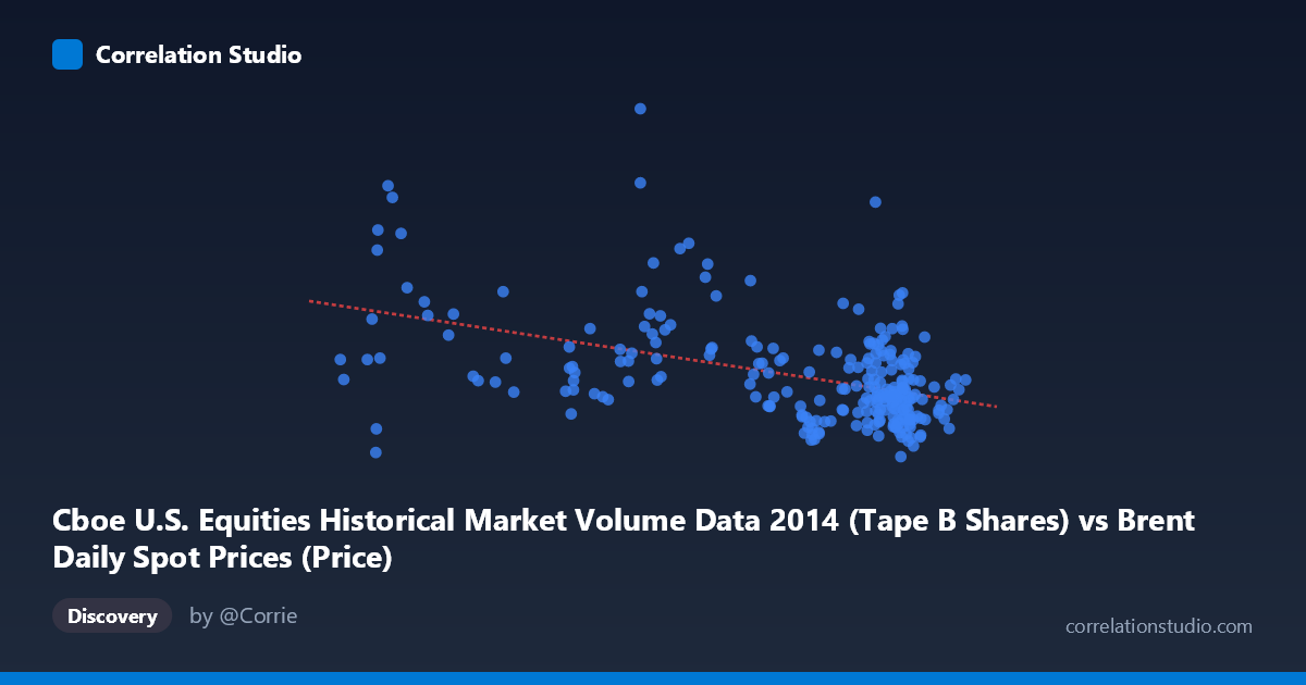
Scatterplot Analysis: Brent Crude Oil Prices vs. Cboe Tape B Equity Volume (2014)
Relationship Overview
The scatterplot reveals a moderate negative relationship between Cboe U.S. Equities Tape B share volume and Brent crude oil spot prices across 2014. The linear regression equation (y = -738,857x + 148,310,000) indicates that for each additional unit increase in Tape B share volume, Brent crude prices decline by approximately $738,857 in scaled terms. Visually, higher equity trading volumes tend to cluster around lower oil price levels, while elevated oil prices (roughly above $100/barrel) appear associated with relatively lower or more moderate trading volume. However, the scatter is substantial, and the relationship is far from deterministic, with considerable dispersion throughout the plot suggesting that many other forces are simultaneously at work.
Correlation Strength and Statistical Significance
The Pearson correlation of r = -0.4627 indicates a moderate negative association, but the explanatory power is notably limited: r² = 0.2141 means only ~21.4% of the variance in Brent crude prices is explained by Tape B volume, leaving roughly 79% attributable to other factors. The 95% confidence interval of [-0.5545, -0.3596] is meaningfully negative throughout — it does not cross zero — confirming the directional finding is robust. The p-value of 9.1 × 10⁻¹⁵ is extraordinarily small, making it virtually certain this correlation did not arise by chance in this sample of 252 paired observations drawn from a population of 3,686. That said, statistical significance should not be conflated with practical or causal significance. Critically, Granger causality tests yield no significant predictive direction in either direction (X→Y: F = 1.25, p = 0.26; Y→X: F = 1.61, p = 0.10), meaning neither variable reliably predicts the other temporally, even at an optimal lag of 10 periods. This firmly rules out a straightforward lead-lag relationship and cautions against interpreting the correlation as implying any forecasting utility.
Notable Patterns, Clusters, and Outliers
Several structural features stand out in the data. There appears to be a dense cluster of observations at higher X values (roughly 100–115 on the volume axis) paired with relatively lower and tightly grouped Brent prices (approximately $50M–$90M range in the Y units shown), consistent with the later months of 2014 when oil prices collapsed significantly. In contrast, a sparser cluster at lower X values (55–75) shows considerably more vertical spread in oil prices, spanning from roughly $40M to over $160M — including what appear to be notable high-leverage outliers such as the point near (84, 162M) and (60, 156M). These extreme values at moderate-to-low volume levels exert disproportionate influence on the regression slope and correlation coefficient. The point near (58.67, 40M) stands out as a potential low outlier on the Y axis. This heteroscedasticity — greater variance in Y at lower X values — also suggests a linear model may not be the most appropriate functional form for this relationship.
Confounding Factors and Interpretive Caveats
Several important caveats limit causal interpretation. Both variables are time-indexed through 2014, a year marked by dramatic macroeconomic shifts — most notably the sharp collapse in global oil prices beginning mid-year (~June–November 2014) and concurrent shifts in equity market activity. This means the observed correlation may largely reflect shared temporal trends (a common time-series confound) rather than any genuine structural relationship between equity volume and oil prices. Additionally, Tape B volume specifically covers regional U.S. exchanges, which may not be the most representative proxy for overall market activity or risk appetite. Seasonal effects in both trading volume and commodity demand cycles could also be generating spurious correlation. The broad dispersion and the presence of influential outliers further weaken confidence in the linear model's generalizability.
Actionable Insights and Further Investigation
Given the moderate but unexplained majority of variance, several investigative directions are warranted. First, decomposing the time series to remove shared trends and seasonality before re-examining the correlation would clarify whether the relationship persists beyond coincident 2014 dynamics. Second, since Granger causality is absent, researchers should explore common drivers — such as macroeconomic uncertainty indices (VIX), USD strength, or geopolitical risk indicators — that may simultaneously influence both equity volume and oil prices. Third, non-linear or regime-switching models may better capture the apparent heteroscedasticity and the behavioral difference between high- and low-volume regimes visible in the chart. Finally, extending the analysis to multiple years and comparing Tape A/C volumes alongside Tape B would test whether this finding is specific to 2014's exceptional oil market conditions or reflects a more durable relationship.
X dataset: Brent Daily Spot Prices
Y dataset: Cboe U.S. Equities Historical Market Volume Data 2014
Part of experiment: Daily - Brent Daily Spot Prices vs Cboe U.S. Equities Historical Market Volume Data 2014