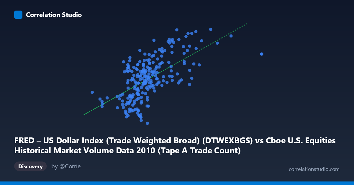
FRED – US Dollar Index (Trade Weighted Broad) (DTWEXBGS) vs Cboe U.S. Equities Historical Market Volume Data 2010 (Tape A Trade Count)
- Pearson correlation (r)
- 0.6215
- Spearman correlation
- 0.6197
- p-value
- 0
- Sample size (n)
- 245
- 95% confidence interval
- 0.5381 to 0.6928
- Granger causality
- None
- Granger optimal lag
- 1
AI analysis
Scatterplot Analysis: US Dollar Index vs. Cboe Tape A Trade Count (2010)
Relationship Overview The scatterplot reveals a positive relationship between the US Dollar Index (Trade Weighted Broad) and the Cboe Tape A Trade Count across 2010 trading days. As the dollar index increases, trade counts tend to rise as well. The linear regression equation (y = 3.04×10⁻⁶x + 89.04) confirms this upward slope, though the scatter around the regression line is substantial, indicating that the relationship, while real, is far from deterministic. The data spans a meaningful X range (roughly 379K to 3.2M in notional volume units) and a comparatively narrow Y range (~89 to 97.6 in trade count index units), which visually compresses the relationship but does not diminish its statistical significance.
Correlation Strength and Statistical Framing The Pearson correlation of r = 0.6215 indicates a moderate-to-strong positive association, but the more sobering figure is r² = 0.3862 — meaning only 38.6% of the variance in Tape A Trade Count is explained by the Dollar Index. This leaves over 61% of variation attributable to other factors entirely. The 95% confidence interval of [0.538, 0.693] is reasonably tight given N = 3,302, and the p-value of effectively zero confirms the relationship is not a statistical artifact. However, the Granger causality results complicate the narrative significantly: neither direction shows significant temporal predictability at conventional thresholds (X→Y: F = 0.19, p = 0.66; Y→X: F = 3.71, p = 0.055). The Y→X direction approaches but misses significance at α = 0.05, hinting weakly that trade count activity may marginally anticipate dollar movements, but this should not be overstated. In practical terms, knowing today's dollar index does not reliably help forecast tomorrow's trade count, and vice versa.
Patterns, Clusters, and Outliers Several notable features emerge from the sample points. There is a visible concentration of observations in the X range of roughly 900K–1.6M paired with Y values between 90–95, forming the dense core of the distribution. Above X ≈ 1.8M, a distinct upper cluster appears with consistently elevated Y values (95–97.5), including standout points like (2,363,720, 97.55), (1,796,427, 97.50), and (2,114,898, 97.34). These high-volume, high-trade-count days likely correspond to specific market events or volatility episodes in 2010 (e.g., the May Flash Crash period). At the low end, the point (508,819, 91.20) stands out as an isolated low-X observation, potentially a holiday-shortened session or an anomalous low-liquidity day. The relationship also appears to show mild heteroscedasticity — variance in Y seems to increase at higher X values — which could slightly inflate the apparent correlation.
Confounding Factors and Caveats Several important caveats apply. First, both variables are time series from the same calendar year (2010), meaning shared temporal trends — such as post-crisis market recovery, seasonality, or macroeconomic cycles — could be driving the co-movement rather than any direct economic link between dollar strength and equity trade volume. Second, the axis labels appear transposed in the dataset metadata (each variable is listed under the other's dataset), which warrants careful verification before drawing firm conclusions. Third, the dollar index is a daily nominal index reflecting broad currency movements, while Tape A trade counts reflect a specific exchange segment; aggregation mismatches could introduce noise. Finally, omitted variables such as VIX (volatility), S&P 500 returns, or Federal Reserve policy announcements are plausible common drivers of both series simultaneously.
Actionable Insights and Further Investigation Given the moderate correlation and absence of Granger causality, this relationship is better treated as a coincident indicator than a predictive one. Practitioners should avoid building trading or risk models that assume dollar index levels forecast near-term equity trade activity. For further investigation, it would be valuable to: (1) partial out shared time trends using detrending or first-differencing to test whether the correlation is spurious; (2) expand the time window beyond 2010 to assess whether this r ≈ 0.62 relationship is stable or specific to post-crisis dynamics; (3) incorporate VIX and market event flags (e.g., Flash Crash dummy) to test whether the high-X, high-Y cluster drives most of the correlation; and (4) re-examine the Y→X Granger result at lags 2–5, since the near-significant p = 0.055 at lag 1 suggests a marginally predictive signal from trade activity to dollar movements that could be worth isolating in a more granular model.
X dataset: Cboe U.S. Equities Historical Market Volume Data 2010
Y dataset: FRED – US Dollar Index (Trade Weighted Broad)
Part of experiment: Daily - Cboe U.S. Equities Historical Market Volume Data 2010 vs FRED – US Dollar Index (Trade Weighted Broad)