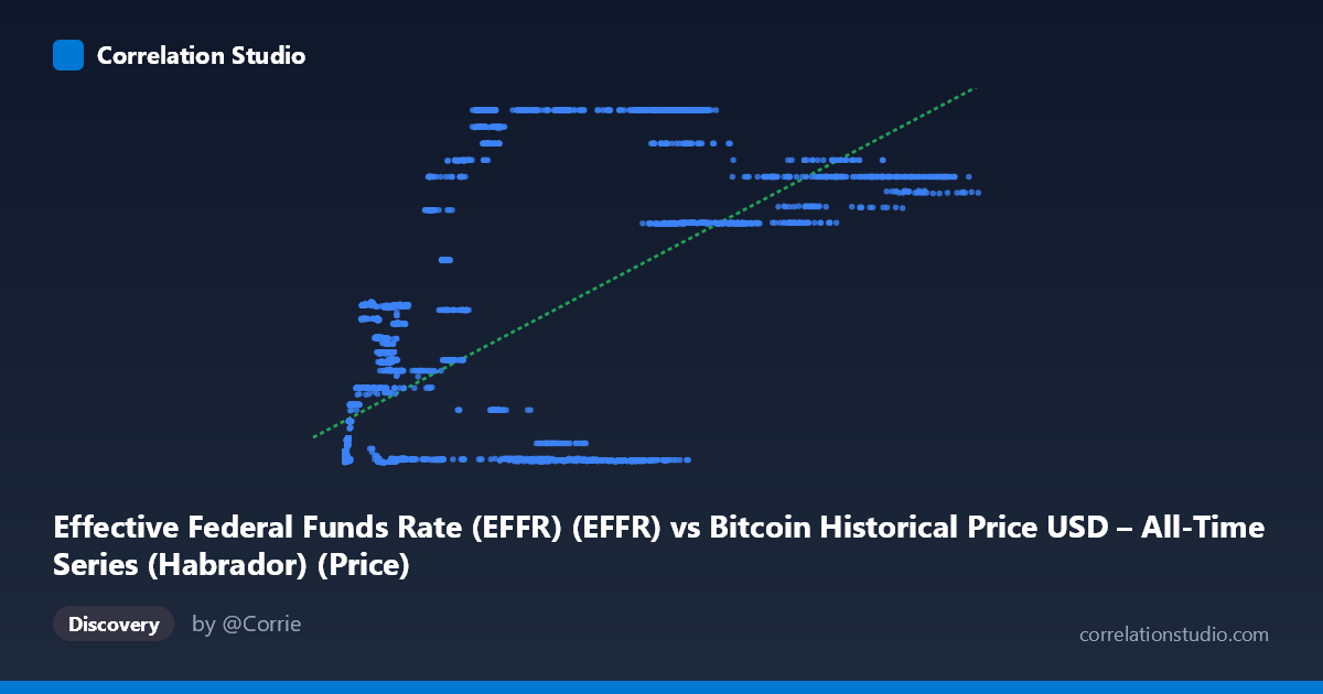
Effective Federal Funds Rate (EFFR) (EFFR) vs Bitcoin Historical Price USD – All-Time Series (Habrador) (Price)
- Pearson correlation (r)
- 0.6631
- Spearman correlation
- 0.5055
- p-value
- 0
- Sample size (n)
- 3963
- 95% confidence interval
- 0.6453 to 0.6802
- Granger causality
- None
- Granger optimal lag
- 1
AI analysis
Analysis of Bitcoin Price vs. Effective Federal Funds Rate
Note on axis labeling: The axis labels appear swapped in the metadata — the data actually shows X = Bitcoin price (range 0.05 to 124,720, consistent with BTC's historical USD range) and Y = EFFR (range 0.04 to 5.33%, consistent with Fed funds rate bounds). The analysis below treats X as Bitcoin price and Y as the federal funds rate, matching the actual data ranges.
1. What the Visualization Reveals
The scatterplot shows a moderate positive association: as Bitcoin's price has risen over its history, the Effective Federal Funds Rate has tended to be higher as well. This is somewhat counterintuitive from a pure macro-finance perspective, since conventional wisdom suggests higher rates (tighter monetary policy) should suppress speculative risk assets like Bitcoin. The pattern here is better understood as two independent long-run trends — Bitcoin's secular price appreciation and the Fed's rate-hiking cycles (particularly 2022-2023) — that happen to overlap in time rather than a signal of direct mechanical linkage.
2. Strength, Direction, and Uncertainty
The correlation coefficient (r = 0.663, r² = 0.440) indicates a moderate positive relationship, with only about 44% of the variance in the Fed funds rate explained by Bitcoin price levels (and vice versa, since correlation is symmetric) — leaving the majority of variance (56%) attributable to other factors. The 95% CI [0.645, 0.680] is tight, and the p-value of ~0 confirms this correlation is highly statistically significant and not due to chance, aided by the large sample size (n=3,963). However, statistical significance here reflects the reliability of the association, not causal strength — with a moderate r², this is a real but far-from-deterministic relationship. Critically, the Granger causality tests show no significant predictive direction in either direction (X→Y: p=0.212; Y→X: p=0.325). This means neither variable's past values reliably help forecast the other's future movements at a 1-period lag — undermining any interpretation that Fed policy changes are driving Bitcoin price (or vice versa) in a lagged, predictive sense.
3. Notable Patterns and Outliers
The scatter shows a distinctive fan/cluster structure rather than a clean linear band. Many low-price Bitcoin points (X < 1,000) cluster tightly at low Y values (~0.05-0.10), reflecting the 2010-2015 near-zero-rate era coinciding with Bitcoin's infancy. A separate cluster appears at high X values (30,000-125,000) paired with high Y values (~3.9-5.3), corresponding to 2022-2024 when Bitcoin reached new highs during the Fed's aggressive hiking cycle. Notably, there's also a cluster of high-X, low-Y points (e.g., X≈47,000-93,000 with Y≈0.06-0.09), representing 2020-2021 when Bitcoin rallied hard under near-zero rates — this scatter directly contradicts a simple linear story and suggests regime-dependent behavior rather than a stable functional relationship.
4. Confounding Factors and Caveats
This is a classic case of spurious correlation via a shared time trend. Both series are non-stationary and have exhibited strong secular drift over the 2010-2026 window — Bitcoin due to adoption/speculative cycles, EFFR due to discrete Fed policy regimes (ZIRP 2008-2015, ZIRP 2020-2022, hiking 2022-2023). Correlating two trending time series without differencing or detrending routinely produces inflated r values that don't reflect genuine bivariate dependence. The lack of Granger causality reinforces that this is likely a coincidental trend alignment rather than a mechanistic link. Other confounders include overall market liquidity conditions, inflation expectations, risk-on/risk-off sentiment cycles, and Bitcoin-specific halving cycles — none of which are controlled for in this simple bivariate analysis.
5. Actionable Insights
Analysts should avoid treating this r²=0.44 as evidence of a tradeable or economically meaningful relationship. Recommended next steps: (1) re-run correlation on differenced or log-return series (ΔBTC vs. ΔEFFR) to test for genuine co-movement stripped of trend; (2) segment the analysis by discrete rate regimes (ZIRP vs. hiking cycles) to test for regime-conditional relationships rather than a single pooled r; (3) incorporate control variables like real yields, DXY (dollar index), or equity risk premiums, which are more theoretically linked to Bitcoin's risk-asset behavior; and (4) given the null Granger result, deprioritize using EFFR as a short-term predictive signal for BTC price and instead focus on longer-horizon macro liquidity indicators (M2 growth, Fed balance sheet changes) that have more established transmission channels to crypto asset prices.
X dataset: Bitcoin Historical Price USD – All-Time Series (Habrador)
Y dataset: Effective Federal Funds Rate (EFFR)
Part of experiment: Bitcoin - Bitcoin Historical Price USD – All-Time Series (Habrador) vs Effective Federal Funds Rate (EFFR)