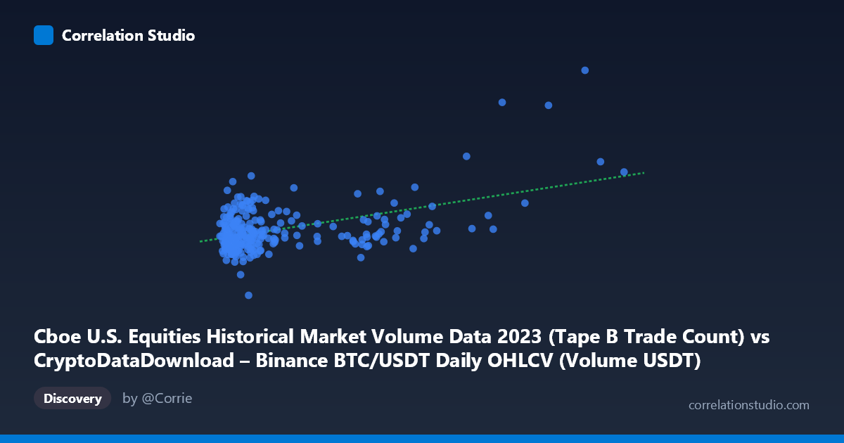
Cboe U.S. Equities Historical Market Volume Data 2023 (Tape B Trade Count) vs CryptoDataDownload – Binance BTC/USDT Daily OHLCV (Volume USDT)
- Pearson correlation (r)
- 0.4803
- Spearman correlation
- 0.2305
- p-value
- 0
- Sample size (n)
- 250
- 95% confidence interval
- 0.3788 to 0.5704
- Granger causality
- None
- Granger optimal lag
- 10
- Time coverage
- 2023-01-03 to 2023-12-29
AI analysis
Analysis: Trade Count vs. Volume Relationship
1. What the Visualization Reveals
The scatterplot shows a moderate positive relationship between two market activity metrics that, despite their labeled column names, appear to both derive from the same underlying BTC/USDT dataset (the axis labels are cross-referenced/swapped between the two dataset descriptions). The data is heavily right-skewed on the X-axis: the vast majority of points cluster below 3 billion, while a handful of extreme values (8.6B, 13.3B, 9.1B, 7B+) stretch the range out to nearly 17.5 billion. This creates a classic "comet" shape — dense clustering at low-to-mid X values with a long thinning tail at high X values.
2. Strength, Direction, and Statistical Confidence
The correlation coefficient (r = 0.48) indicates a moderate positive relationship, but r² = 0.231 tells the more important story: only about 23% of the variance in Y is explained by X, leaving roughly 77% attributable to other factors or noise. The 95% CI [0.379, 0.570] is reasonably tight and entirely positive, and the p-value (8.88E-16) confirms this correlation is highly statistically significant — not a fluke of sampling. However, statistical significance with n=250 (drawn from a population of 3,212) does not imply strong predictive power; a moderate r² means this relationship has limited standalone utility for forecasting.
Critically, the Granger causality tests show no significant predictive direction in either direction (X→Y: p=0.66; Y→X: p=0.97). This means that even though the two series are correlated contemporaneously, neither variable's past values help forecast the other's future values better than the other's own history. This is an important distinction: correlation here reflects synchronous co-movement (likely both driven by overall market volume/activity levels on given days), not a lead-lag causal structure.
3. Notable Patterns and Outliers
The bulk of points sit in a tight band between X = 500M–3B and Y = 330K–500K, forming the core linear trend. Several notable outliers deserve attention: - One point at (1,688,715,728, 182,084) is a clear low-Y outlier, sitting far below the trend line despite a modest X value. - High-X points (13.3B, 9.1B, 8.6B) show Y values that don't scale proportionally — e.g., the 13.3B point yields Y≈511K, while the 8.6B point yields only Y≈349K, suggesting the relationship flattens or becomes noisy at the extremes. - A slight fan/heteroscedasticity pattern is visible: variance in Y appears to increase somewhat at low-to-mid X values (e.g., 1.9B point at Y=534,900 vs. similar X values near 340K–430K), suggesting the linear model may not capture the full complexity of the relationship.
4. Confounding Factors and Caveats
Several caveats limit interpretation: - Dataset labeling confusion: The axis descriptions suggest both columns trace back to Binance BTC/USDT OHLCV data, with Cboe equities volume mentioned only in dataset metadata, not axis content — this cross-referencing raises questions about whether this is a true cross-market comparison or an artifact of mismatched labels. - Time-series autocorrelation: Daily financial/volume data are typically autocorrelated (trending, volatility clustering), which can inflate apparent correlation between two unrelated series (spurious correlation risk). - Non-stationarity: Both series likely have trends/seasonality across 2023 (e.g., BTC volume spikes during specific events) that could drive co-movement without genuine causal linkage. - Skewed X distribution: The extreme right tail (values 5B) may be exerting outsized leverage on the regression slope; a log transformation would likely be more appropriate.
5. Actionable Insights
1. Verify data provenance — confirm whether X and Y genuinely represent independent markets or overlapping/derived Binance metrics before drawing cross-market conclusions. 2. Apply log transformation to X (and possibly Y) given the extreme skew, then re-run correlation/regression — this will likely improve model fit and reduce leverage from outliers. 3. Since no Granger causality exists, avoid using either series to forecast the other in a trading or predictive model; treat the relationship as contemporaneous/coincidental co-movement rather than a lead indicator. 4. Investigate the low-Y outlier (Y=182,084) — check if it corresponds to a specific date (holiday, exchange outage, data error) that warrants exclusion or special handling. 5. Test for a threshold/nonlinear effect at high X values (5B), where the linear relationship appears to break down — a piecewise or log-log model may better represent behavior across the full range.
X dataset: CryptoDataDownload – Binance BTC/USDT Daily OHLCV
Y dataset: Cboe U.S. Equities Historical Market Volume Data 2023
Part of experiment: Bitcoin - CryptoDataDownload – Binance BTC/USDT Daily OHLCV vs Cboe U.S. Equities Historical Market Volume Data 2023