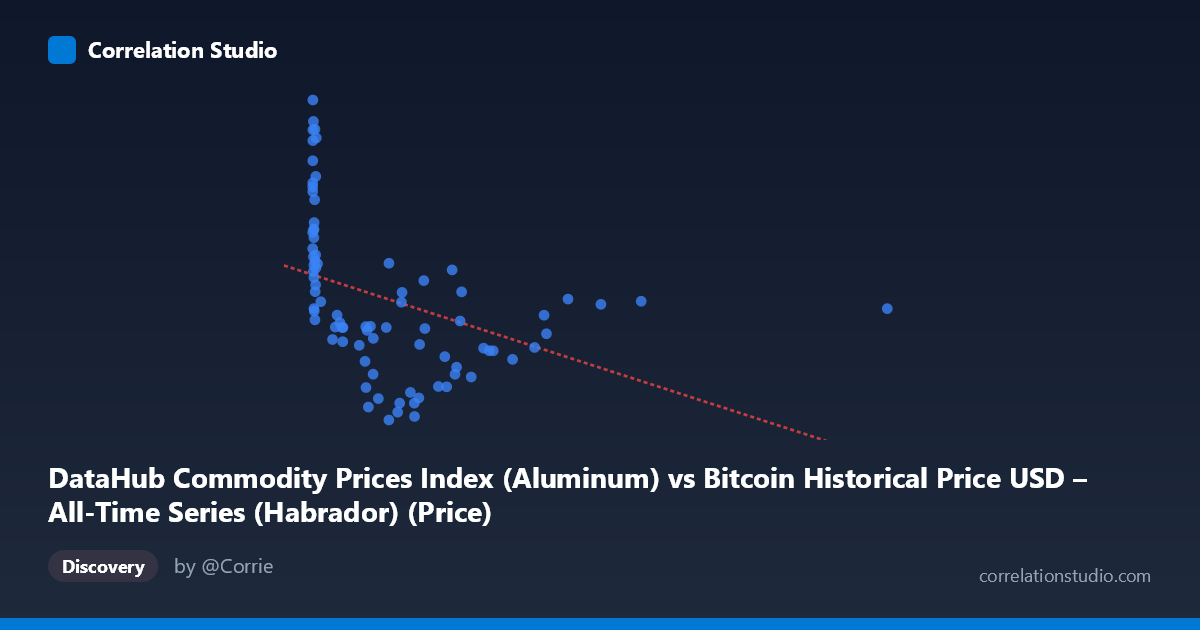
DataHub Commodity Prices Index (Aluminum) vs Bitcoin Historical Price USD – All-Time Series (Habrador) (Price)
- Pearson correlation (r)
- -0.4008
- Spearman correlation
- -0.661
- p-value
- 0.000174
- Sample size (n)
- 83
- 95% confidence interval
- -0.5674 to -0.2026
- Granger causality
- None
- Granger optimal lag
- 10
- Time coverage
- 2010-08-01 to 2017-06-01
AI analysis
Analysis: Aluminum Commodity Prices Index vs. Bitcoin Historical Price USD
1. Overview of the Relationship
The scatterplot displays a moderate negative correlation between the Aluminum Commodity Price Index (X-axis) and Bitcoin price in USD (Y-axis). The data shows a clear concentration of points at low X-values (below 500), with Bitcoin prices ranging widely (roughly 1,450–2,660) in this cluster, while a sparser tail of higher X-values (up to 2,452) corresponds to Bitcoin prices that stabilize in a narrower band (~1,700–1,950). This pattern suggests the relationship is not uniformly linear across the full range of X.
2. Strength, Direction, and Statistical Confidence
The Pearson correlation coefficient of r = -0.40 indicates a moderate negative linear relationship, meaning that as the aluminum price index increases, Bitcoin prices tend to decrease somewhat. However, r² = 0.16 reveals that only about 16% of the variance in Bitcoin price is explained by aluminum prices — the vast majority (84%) is driven by other factors. The 95% confidence interval [-0.567, -0.203] is entirely negative and reasonably tight, and the p-value (0.000174) is highly significant, giving strong confidence that a real (non-zero) negative association exists in this sample — but the practical explanatory power remains modest. Critically, the Granger causality tests show no significant predictive direction in either direction (X→Y: p=0.955; Y→X: p=0.430), meaning neither variable meaningfully helps forecast the other's future values at the tested lags. This strongly suggests the correlation is likely coincidental, driven by a shared time trend or external confound, rather than a genuine causal or predictive linkage.
3. Notable Patterns and Features
The data reveals a distinctive clustering pattern: the majority of points sit at very low aluminum index values (near 0–50), corresponding to a wide vertical spread of Bitcoin prices — including several high-value outliers (Bitcoin 2,300 near X≈0–15). This vertical "fan" at low X suggests that when aluminum prices are low, Bitcoin price is highly variable and not well predicted by X at all. As X increases beyond ~500, Bitcoin prices compress into a tighter, lower range (~1,700–1,950), producing an apparent downward slope that may be more an artifact of range restriction than a true linear trend. The note that Spearman ρ exceeds Pearson r reinforces that a monotonic but non-linear (e.g., logarithmic or power-law) relationship fits better — consistent with the compressed/asymptotic behavior at high X.
4. Confounding Factors and Caveats
This is a classic setup for spurious correlation via time-trend confounding: both series span 2010–2017, a period when Bitcoin grew from near-zero to major bull-market territory, while global commodity indices (including aluminum) underwent independent cyclical trends (e.g., the 2011–2016 commodities slump). Any two time series with their own secular trends can show statistically significant correlation without any causal mechanism connecting them. Sample size asymmetry (n=83 paired vs. N=449 population) and uneven X-distribution (heavily skewed toward low values with few high-leverage points 1000) mean the regression slope is disproportionately influenced by a handful of observations. The lack of Granger causality is the strongest evidence that this is not a functional economic relationship.
5. Recommendations for Further Investigation
Given the non-significant Granger causality and modest r², this correlation should not be used for predictive or trading purposes. To clarify whether a real relationship exists, analysts should: (1) detrend or difference both series (e.g., use returns/percentage changes rather than levels) to remove shared time-trend effects before re-testing correlation; (2) fit and compare logarithmic or power-law models given the Spearman/Pearson discrepancy; (3) test for cointegration rather than simple correlation, given both are non-stationary price series; and (4) investigate a plausible macroeconomic confound (e.g., USD strength, global risk sentiment, or Chinese industrial demand) that could independently drive both aluminum prices and Bitcoin's speculative valuation.
X dataset: Bitcoin Historical Price USD – All-Time Series (Habrador)
Y dataset: DataHub Commodity Prices Index
Part of experiment: Bitcoin - Bitcoin Historical Price USD – All-Time Series (Habrador) vs DataHub Commodity Prices Index