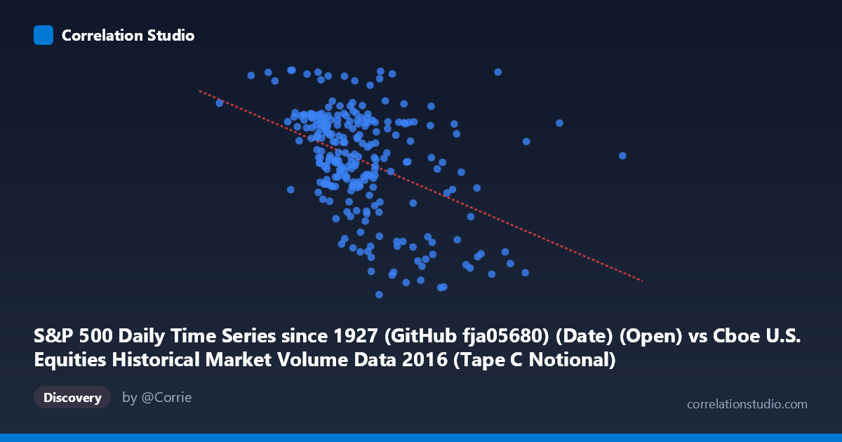
S&P 500 Daily Time Series since 1927 (GitHub fja05680) (Date) (Open) vs Cboe U.S. Equities Historical Market Volume Data 2016 (Tape C Notional)
- Pearson correlation (r)
- -0.4361
- Spearman correlation
- -0.4241
- p-value
- 0
- Sample size (n)
- 252
- 95% confidence interval
- -0.5311 to -0.3304
- Granger causality
- None
- Granger optimal lag
- 1
AI analysis
Scatterplot Analysis: S&P 500 Date vs. Cboe Tape C Notional Value (2016)
Relationship Overview
The scatterplot reveals a negative relationship between the S&P 500 trading date (expressed as a Unix timestamp on the X-axis) and the Cboe Tape C Notional trading volume on the Y-axis. As the year 2016 progresses, Tape C Notional values show a general tendency to decline, though with considerable scatter throughout. The linear regression equation (y = -3.87E-08x + 2286.78) captures this downward drift, but the wide dispersion of points around the regression line immediately signals that time alone is a weak predictor of notional volume. Visually, the data forms a broad, diffuse cloud with a modest downward tilt rather than a tight, well-defined linear band.
Correlation Strength and Statistical Significance
The Pearson correlation of r = -0.4361 indicates a moderate negative association, but the coefficient of determination r² = 0.1902 is the more sobering figure — time explains only ~19% of the variance in Tape C Notional values, leaving roughly 81% attributable to other factors. The 95% confidence interval of [-0.5311, -0.3304] is meaningfully bounded away from zero, and the extremely small p-value (3.999E-13) confirms this is not a chance finding given the sample of 252 paired observations drawn from a population of 3,622. However, statistical significance here is heavily amplified by sample size and should not be mistaken for practical or economic significance. Critically, the Granger causality tests show no significant predictive directionality in either direction (X→Y: F=0.453, p=0.502; Y→X: F=0.274, p=0.601), meaning that knowing the date does not help forecast next-period notional volume beyond its own history, and vice versa. This effectively rules out a meaningful temporal lead-lag relationship between these two variables.
Patterns, Clusters, and Outliers
Several features stand out beyond the overall trend. There appears to be a cluster of high-notional observations (Y 2,150) concentrated in the mid-range of the X-axis, roughly corresponding to mid-year 2016, suggesting a period of elevated trading activity. Conversely, notable low-notional outliers are visible at higher X values (later in 2016), with some points dipping well below 1,900 — consistent with the lower-volume drift seen in late-year equity markets. One point near the far left of the X-axis (approximately 3.47B timestamp, Y ≈ 2,270) stands out as an extreme high-notional observation early in the year, possibly reflecting the January 2016 market turbulence that drove elevated volume. A few isolated high-X, low-Y points (e.g., ~7.3B timestamp, Y ≈ 1,885) appear as potential outliers that may disproportionately influence the regression slope.
Confounding Factors and Caveats
Several important caveats apply. First, the X-axis encodes calendar time, not a continuous financial variable, so the "correlation" largely captures secular intra-year volume trends (e.g., summer lulls, year-end slowdowns) rather than a causal mechanism. Second, market microstructure events in 2016 — including the Brexit vote (June), U.S. presidential election (November), and Federal Reserve rate decisions — likely drove episodic volume spikes that appear as outliers rather than systematic trends. Third, the Tape C designation refers specifically to NYSE Arca-listed securities, meaning this is a subset of total market volume, and its dynamics may differ from broad market behavior. Finally, the dataset's N of 3,622 vs. a sample of 252 raises questions about whether the sampled points fully represent the distributional tails, and the timestamp encoding of dates introduces artificial precision into what is fundamentally a discrete daily variable.
Actionable Insights and Further Investigation
Given that time explains only 19% of Tape C Notional variance with no Granger-causal pathway, practitioners should avoid using calendar position alone as a volume forecasting input. More productive next steps would include: (1) regressing Tape C Notional against VIX or realized volatility, which are known volume drivers, to assess whether volatility explains the residual 81%; (2) decomposing the time series seasonally to isolate day-of-week, month-of-year, and holiday effects that the raw timestamp obscures; (3) examining the high-leverage outliers individually to determine whether they correspond to identifiable macro events, which could motivate an event-study design; and (4) extending the analysis across multiple years to determine whether this intra-year negative drift is a consistent structural feature of Tape C markets or unique to 2016's specific macro environment.
X dataset: Cboe U.S. Equities Historical Market Volume Data 2016
Y dataset: S&P 500 Daily Time Series since 1927 (GitHub fja05680) (Date)
Part of experiment: Daily - Cboe U.S. Equities Historical Market Volume Data 2016 vs S&P 500 Daily Time Series since 1927 (GitHub fja05680) (Date)