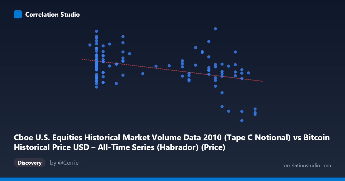
Cboe U.S. Equities Historical Market Volume Data 2010 (Tape C Notional) vs Bitcoin Historical Price USD – All-Time Series (Habrador) (Price)
- Pearson correlation (r)
- -0.4173
- Spearman correlation
- -0.3013
- p-value
- 0.000003
- Sample size (n)
- 117
- 95% confidence interval
- -0.5567 to -0.2551
- Granger causality
- None
- Granger optimal lag
- 10
- Time coverage
- 2010-07-19 to 2010-12-31
AI analysis
Analysis: Cboe Equities Volume vs. Bitcoin Price (2010)
1. Overview of the Relationship
The scatterplot shows a moderate negative linear relationship between the two variables: as the X variable (Cboe U.S. equities market volume) increases, the Y variable (Bitcoin price) tends to decrease. The regression line (y = -3.32×10⁹x + 3.87×10⁹) slopes downward, and points cluster fairly densely in the X range of 0.06–0.10 and 0.19–0.28, with a visible gap between roughly 0.11 and 0.19. This bimodal clustering suggests the underlying data may represent two distinct regimes or time periods rather than a continuous, evenly sampled relationship.
2. Strength, Direction, and Statistical Confidence
The correlation coefficient (r = -0.4173) indicates a moderate negative association, but r² = 0.1741 reveals that only about 17.4% of the variance in Bitcoin price is explained by equities volume — meaning over 82% of the variability is driven by other factors entirely. The 95% confidence interval [-0.5567, -0.2551] is entirely negative and reasonably tight, and the p-value (2.86×10⁻⁶) is highly significant, confirming this is a real, non-random association rather than noise. However, statistical significance should not be conflated with practical predictive power given the low r². Critically, the Granger causality tests show no significant predictive direction in either direction (X→Y: p=0.675; Y→X: p=0.937), meaning past values of one series do not meaningfully help forecast future values of the other. This strongly suggests the correlation is contemporaneous/coincidental rather than causal or lead-lag in nature.
3. Notable Patterns and Outliers
Several features stand out: a tight cluster of high Bitcoin prices (~$4-5B on this scale) at low X values (0.06-0.10), and a cluster of lower, more volatile prices at higher X values (0.19-0.28), including a steep drop-off at X=0.30 where prices fall to ~$1.5-1.7B — among the lowest in the dataset. There's also a notable outlier at X=0.24 with Y=4.99B, the maximum price value, sitting well above the surrounding points at similar X values. The relationship appears possibly non-linear or regime-shifting rather than strictly linear — the low-X cluster shows high variance (2.6B-4.7B) while the high-X region shows a more gradual decline, with the X=0.30 points forming a distinct low-price tail.
4. Confounding Factors and Caveats
The most important caveat is that this compares two datasets described inconsistently — the axis labels swap the source datasets (X is labeled as Bitcoin price data description while actually containing Cboe volume, and vice versa), suggesting possible metadata mismatch that warrants verification before drawing conclusions. Both series are also likely non-stationary time series (Bitcoin price trended strongly in 2010; equity volumes have their own trends/seasonality), which can produce spurious correlations when two trending series are compared without differencing or detrending. Additionally, N=3,302 (full population) vs. n=117 (sampled pairs) indicates substantial subsampling — results may be sensitive to which 117 points were selected, especially with clustered/gapped X-coverage.
5. Recommendations for Further Investigation
Given the lack of Granger causality and modest r², treat this as a weak contemporaneous association rather than a predictive relationship — it should not be used for forecasting one series from the other. Recommended next steps: (1) verify the axis/dataset labeling to ensure the comparison is what's intended; (2) test the relationship on differenced or log-returns data to rule out spurious correlation from shared trends; (3) investigate the X=0.11–0.19 gap and the X=0.30 outlier cluster to understand whether they represent distinct market regimes (e.g., specific weeks/events in late 2010); and (4) explore whether a third factor (e.g., overall market risk sentiment, dollar liquidity, or date/time itself) drives both series independently, producing a confound rather than direct interaction.
X dataset: Bitcoin Historical Price USD – All-Time Series (Habrador)
Y dataset: Cboe U.S. Equities Historical Market Volume Data 2010
Part of experiment: Bitcoin - Bitcoin Historical Price USD – All-Time Series (Habrador) vs Cboe U.S. Equities Historical Market Volume Data 2010