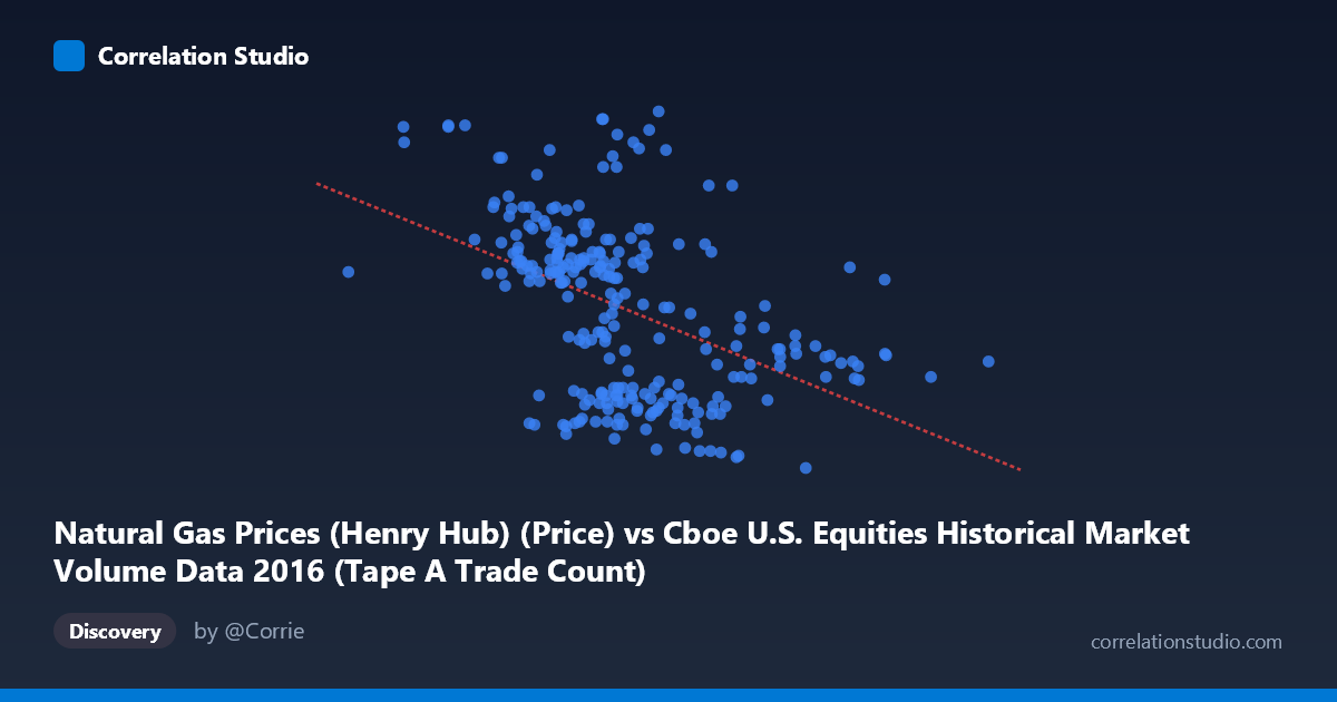
Natural Gas Prices (Henry Hub) (Price) vs Cboe U.S. Equities Historical Market Volume Data 2016 (Tape A Trade Count)
- Pearson correlation (r)
- -0.4565
- Spearman correlation
- -0.4936
- p-value
- 0
- Sample size (n)
- 252
- 95% confidence interval
- -0.5491 to -0.3528
- Granger causality
- None
- Granger optimal lag
- 1
AI analysis
Scatterplot Analysis: Natural Gas Prices vs. Cboe Equity Trade Count (2016)
Relationship Overview The scatterplot reveals a negative relationship between Henry Hub natural gas spot prices (X-axis) and Cboe U.S. equities tape A trade counts (Y-axis) across 252 trading days in 2016. As natural gas prices increase, equity trade counts tend to decrease, and vice versa. The linear regression equation (y = -8.62E-07x + 3.715) confirms this inverse trend, though the scatter around the regression line is visually substantial, suggesting the relationship — while statistically real — is far from deterministic. The data spans a natural gas price range from roughly $1.49 to $3.80, capturing meaningful price variation across the year, while trade counts cluster predominantly between approximately 1.75 and 3.25 million trades.
Correlation Strength and Statistical Interpretation The Pearson correlation of r = -0.4565 indicates a moderate negative association, but the more practically meaningful figure is r² = 0.2084 — meaning natural gas prices explain only about 20.8% of the variance in equity trade counts. The remaining ~79% of variability is driven by other factors entirely. The 95% confidence interval for r of [-0.5491, -0.3528] is reassuringly tight and does not cross zero, indicating reasonable precision in the estimate. The p-value of 2.24 × 10⁻¹⁴ is highly significant given n = 252, confirming this is extremely unlikely to be a chance finding. However, Granger causality tests in both directions fail to reach significance (X→Y: F = 0.868, p = 0.352; Y→X: F = 0.599, p = 0.440), meaning neither variable reliably predicts the other one period ahead in time. This is a critical caveat: the correlation is real but neither variable leads the other temporally, undermining any causal interpretation.
Notable Patterns, Clusters, and Outliers The sample points reveal several noteworthy features. Trade counts appear somewhat bimodally distributed — many observations cluster near lower values (~1.77–2.00 million) and another group clusters near higher values (~2.69–3.06 million), potentially reflecting distinct market regimes or seasonal trading patterns. A handful of outliers are visible at the extremes: notably one observation at approximately (1,000,524; 3.50) and another at (1,428,849; 3.56) represent unusually high trade counts, while very high natural gas prices (above ~$2.2M on the X scale) consistently pair with lower trade counts near 2.15–2.30. The spread of Y values at any given X is wide, reinforcing the modest explanatory power. There is no strong evidence of non-linearity, though the relationship may taper at extreme price values.
Confounding Factors and Caveats Several important caveats apply. First, this correlation is almost certainly spurious or driven by shared seasonal confounders: natural gas prices are highest in winter (heating demand) and lowest in summer, while equity trading volumes follow their own calendar patterns driven by earnings seasons, holidays, and market volatility events. Both series are likely independently responding to time-of-year effects rather than causally influencing each other. Second, the dataset is limited to a single calendar year (2016), which is insufficient to distinguish genuine structural relationships from year-specific coincidences. Third, the Cboe Tape A trade count reflects a narrow slice of equity market activity, and results may not generalize to broader volume metrics. Finally, the failure of Granger causality tests strongly suggests that any apparent relationship is contemporaneous and non-directional, likely reflecting common external drivers rather than any meaningful economic linkage between energy prices and equity trading activity.
Actionable Insights and Further Investigation Given the statistically significant but causally uninterpretable correlation, the most productive next steps would be to: (1) control for seasonality in both series using detrending or seasonal decomposition (e.g., STL decomposition) to test whether the correlation persists after removing calendar effects; (2) extend the time series across multiple years to assess whether the r = -0.46 relationship is stable or year-specific; (3) introduce mediating variables such as the VIX (equity volatility index), broader energy market indices, or macroeconomic indicators to identify what might be independently driving both series; and (4) explore whether subsector equity volumes (e.g., energy sector ETFs) show a stronger or more directional relationship with natural gas prices than the broad market Tape A counts, which would be a more theoretically motivated hypothesis. The current finding is best treated as an interesting empirical pattern warranting explanation rather than an actionable trading or risk signal.
X dataset: Cboe U.S. Equities Historical Market Volume Data 2016
Y dataset: Natural Gas Prices (Henry Hub)
Part of experiment: Daily - Cboe U.S. Equities Historical Market Volume Data 2016 vs Natural Gas Prices (Henry Hub)