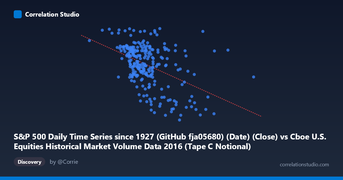
S&P 500 Daily Time Series since 1927 (GitHub fja05680) (Date) (Close) vs Cboe U.S. Equities Historical Market Volume Data 2016 (Tape C Notional)

Pearson correlation (r): -0.4623
Spearman correlation: -0.429
p-value: 0
Sample size (n): 252
95% confidence interval: -0.5542 to -0.3592
Granger causality: None
Granger optimal lag: 4

AI analysis

Analysis: S&P 500 Closing Price vs. Cboe Tape C Notional Volume (2016)

Relationship Overview

The scatterplot reveals a negative relationship between the S&P 500 closing price (X-axis, expressed as a date-encoded numeric value representing trading days across 2016) and Cboe Tape C notional trading volume (Y-axis). As the year progresses — that is, as the date value increases — Tape C notional volume tends to decline. The linear regression equation (y = −4.11×10⁻⁸x + 2299.58) confirms this downward slope, suggesting that notional volume traded on Tape C venues trended lower as S&P 500 prices generally rose throughout 2016. This inverse pattern is consistent with well-documented market microstructure dynamics: rising equity prices in a bull-trending environment tend to be associated with declining volatility and reduced urgency to trade, compressing notional volumes on individual exchange tapes.

Correlation Strength and Statistical Significance

The Pearson correlation of r = −0.4623 indicates a moderate negative association, but the explanatory power is modest: r² = 0.2137, meaning only about 21.4% of the variance in Tape C notional volume is explained by the date-encoded S&P 500 price variable. Roughly 79% of the variation in volume remains unexplained by this single predictor. The 95% confidence interval of [−0.5542, −0.3592] is entirely negative, lending confidence that the direction of the relationship is genuine rather than a sampling artifact, and the p-value of 9.55×10⁻¹⁵ makes this correlation highly statistically significant at any conventional threshold — effectively ruling out chance given a sample of n = 252. However, Granger causality tests find no significant temporal predictive relationship in either direction (X→Y: F = 0.68, p = 0.60; Y→X: F = 1.02, p = 0.40). This is a critical caveat: despite the significant correlation, neither variable reliably predicts future values of the other at a 4-period lag, meaning the relationship is associative and contemporaneous rather than directionally causal in a temporal sense.

Notable Patterns, Clusters, and Outliers

Several features stand out in the sampled data points. There is a visible cluster of high-volume observations (Tape C notional ~2,150–2,270) concentrated at lower date values (roughly early-to-mid 2016, X ≈ 3.4–4.5 billion range), consistent with elevated market activity during the volatile early months of 2016 when global growth fears and oil price crashes drove heavy trading. Conversely, lower-volume readings (Y ≈ 1,830–1,940) tend to appear at higher X values, corresponding to the latter half of 2016. Notable outliers include the point near (3,469,875,424, 2,265) — an exceptionally high notional volume — and several low-volume points near (7,312,471,143, 1,893) and (6,246,205,179, 1,869), which appear to be late-year dates with suppressed Tape C activity. The scatter is wide throughout, reinforcing that the relationship is far from deterministic and that day-to-day volume fluctuations are driven by many factors beyond the date or price level alone.

Confounding Factors and Interpretive Caveats

Several confounds complicate interpretation. First, the X-axis encodes calendar date as a numeric proxy for S&P 500 closing price, which conflates time trends with price levels — it is not entirely clear whether volume is responding to the price level, the passage of time, seasonal effects, or all three simultaneously. Second, 2016 was an atypical year with discrete structural shocks: Brexit (June), the U.S. presidential election (November), and Federal Reserve rate decisions, each of which triggered episodic volume spikes that are not well captured by a linear model. Third, Tape C specifically covers NYSE Arca-listed securities, so shifts in market share across exchanges (e.g., routing behavior changes, maker-taker fee adjustments) could drive volume changes independent of broad market conditions. Finally, the population size (N = 3,622) versus sample (n = 252) gap suggests the full dataset may reveal additional structure not visible in this sample.

Actionable Insights and Further Investigation

Given that the correlation is statistically significant but explains only ~21% of variance with no Granger-causal directionality, practitioners should avoid using this relationship for predictive modeling without additional variables. Recommended next steps include: (1) decomposing the time series to separate secular trend from volatility-driven volume spikes — regressing Tape C volume on the VIX or realized volatility would likely improve explanatory power substantially; (2) examining exchange market share dynamics across Tapes A, B, and C simultaneously to determine whether Tape C volume declines reflect redistribution rather than absolute volume contraction; (3) applying structural break tests around Brexit and the election to assess whether the negative trend holds uniformly or is driven by a few high-leverage episodes; and (4) extending the analysis to multiple years to test whether the 2016 pattern replicates or is idiosyncratic to that year's market regime.

X dataset: Cboe U.S. Equities Historical Market Volume Data 2016

Y dataset: S&P 500 Daily Time Series since 1927 (GitHub fja05680) (Date)

Part of experiment: Daily - Cboe U.S. Equities Historical Market Volume Data 2016 vs S&P 500 Daily Time Series since 1927 (GitHub fja05680) (Date)