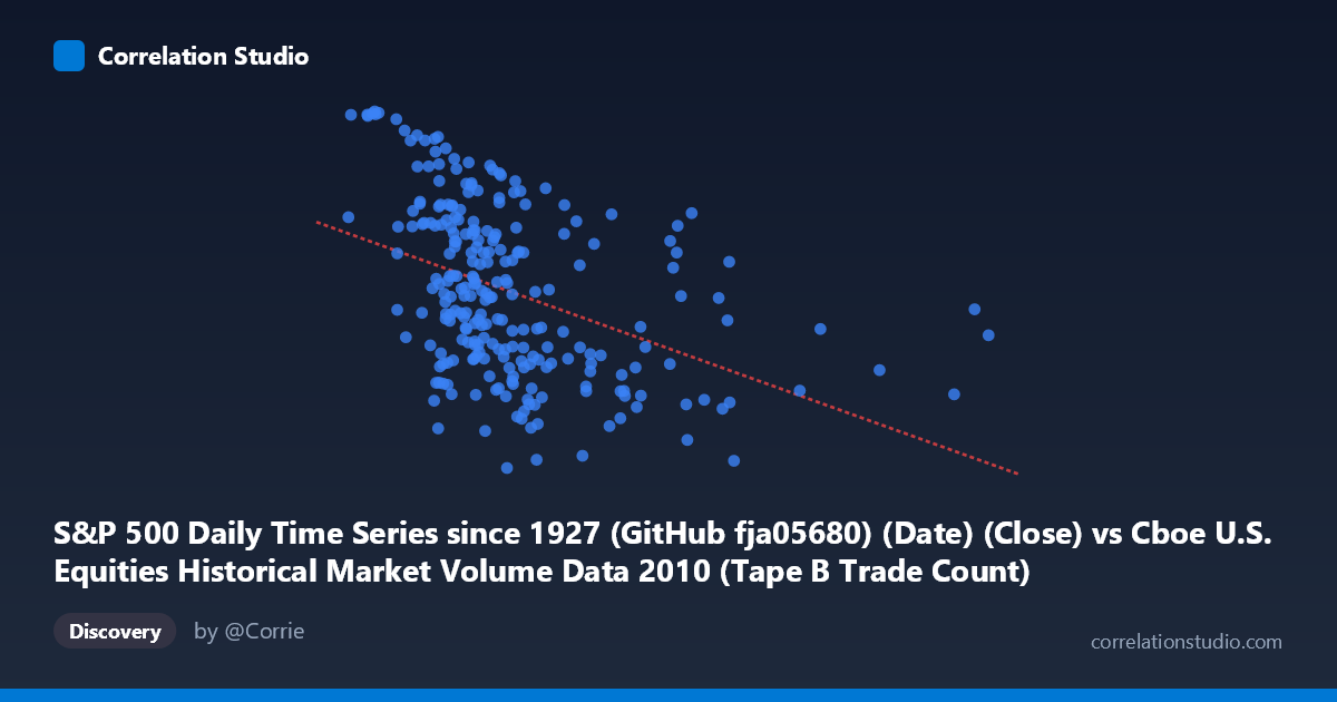
S&P 500 Daily Time Series since 1927 (GitHub fja05680) (Date) (Close) vs Cboe U.S. Equities Historical Market Volume Data 2010 (Tape B Trade Count)

Pearson correlation (r): -0.4188
Spearman correlation: -0.491
p-value: 0
Sample size (n): 252
95% confidence interval: -0.5157 to -0.3113
Granger causality: None
Granger optimal lag: 1

AI analysis

Analysis: S&P 500 Close Price vs. Cboe Tape B Trade Count (2010)

Relationship Overview The scatterplot reveals a negative relationship between the S&P 500 daily closing price (X-axis) and the Cboe Tape B Trade Count (Y-axis) across 252 trading days in 2010. As the S&P 500 close price increases, Tape B trade counts tend to decline, suggesting that higher equity valuations during this period were associated with fewer discrete trades on Cboe's Tape B venues. The linear regression equation (y = −0.000186x + 1,196.35) quantifies this inverse slope, though the relationship is far from deterministic and carries substantial scatter throughout.

Correlation Strength and Statistical Significance The Pearson correlation of r = −0.419 indicates a moderate negative association, but the explanatory power is modest: R² = 0.175, meaning only about 17.5% of the variance in Tape B trade counts is explained by S&P 500 closing price levels. The remaining ~82.5% is attributable to other factors entirely. The 95% confidence interval of [−0.516, −0.311] is comfortably negative and does not cross zero, reinforcing that the direction is reliable. The p-value of 4.01 × 10⁻¹² confirms the correlation is statistically significant well beyond conventional thresholds given the population of N = 3,302. Critically, however, Granger causality tests reveal no significant temporal predictive direction in either direction — X→Y (F = 1.52, p = 0.219) and Y→X (F = 2.87, p = 0.092) both fail conventional significance — meaning neither variable meaningfully predicts the other's future values. This decouples statistical correlation from any practical forecasting utility.

Notable Patterns, Clusters, and Outliers Several structural features stand out in the data. The bulk of observations cluster in the X range of roughly 100,000–450,000 with trade counts spanning 1,050–1,260, forming a moderately downward-sloping core. However, there is a distinct right-side tail of high-volume outliers — including points near 778,566, 918,660, and several in the 500,000–680,000 range — that pull the regression slope but sit well below the main cluster in Tape B counts (~1,062–1,120), consistent with the negative trend. Two notable high-trade-count outliers (≈1,257–1,259) occur at very low X values (~120,757 and ~134,700), reinforcing the inverse pattern. These extremes suggest that low-price/high-volume days and high-price/low-volume days may reflect distinct market regimes rather than a smooth continuum.

Confounding Factors and Caveats Several important caveats temper interpretation. First, the S&P 500 close price is being used as the X-axis, but it functions here essentially as a time proxy — prices trended upward through much of 2010, while trade fragmentation and exchange competition were simultaneously evolving, meaning this correlation may be partly spurious due to shared time trends rather than a direct causal mechanism. Second, Tape B specifically covers NYSE American (AMEX) and regional exchange securities — a subset of total market activity — so the trade count metric does not represent broad market participation. Third, volume and trade count are influenced by algorithmic trading activity, index rebalancing events, and macroeconomic announcements, none of which are controlled for here. The absence of Granger causality further warns against reading economic meaning into the temporal structure.

Actionable Insights and Further Investigation Given the limitations, several avenues merit investigation. Detrending both series (e.g., using first differences or regression residuals against a time index) would test whether the correlation persists independently of the shared upward price drift in 2010. Analysts should also examine whether specific dates corresponding to the extreme outliers (e.g., the ~918,660 and ~120,757 X-values) align with known market events such as the May 6 Flash Crash, which could explain anomalous volume-price divergences. Extending the analysis to Tape A and Tape C trade counts would clarify whether the Tape B pattern is idiosyncratic or systemic. Finally, incorporating VIX or realized volatility as a covariate could both explain additional variance and reveal whether the price–trade count relationship is primarily a volatility-mediated phenomenon, where low-volatility rising markets suppress trade frequency while high-volatility episodes spike it.

X dataset: Cboe U.S. Equities Historical Market Volume Data 2010

Y dataset: S&P 500 Daily Time Series since 1927 (GitHub fja05680) (Date)

Part of experiment: Daily - Cboe U.S. Equities Historical Market Volume Data 2010 vs S&P 500 Daily Time Series since 1927 (GitHub fja05680) (Date)