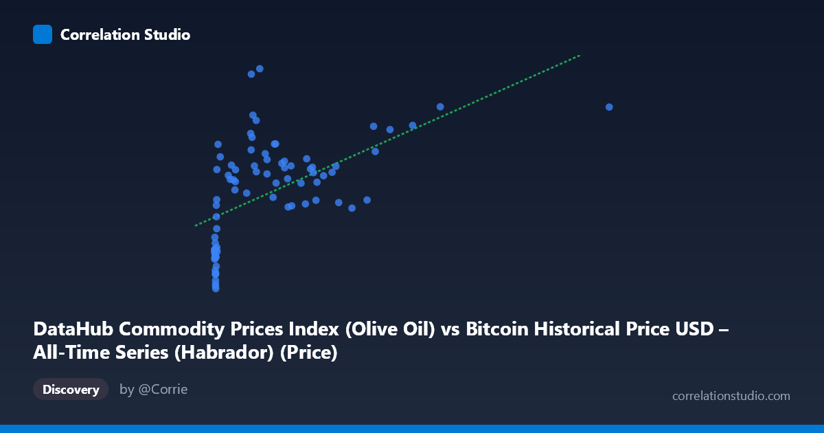
DataHub Commodity Prices Index (Olive Oil) vs Bitcoin Historical Price USD – All-Time Series (Habrador) (Price)
- Pearson correlation (r)
- 0.5557
- Spearman correlation
- 0.6695
- p-value
- 0
- Sample size (n)
- 83
- 95% confidence interval
- 0.3863 to 0.6888
- Granger causality
- None
- Granger optimal lag
- 10
- Time coverage
- 2010-08-01 to 2017-06-01
AI analysis
Analysis: Bitcoin Price vs. Olive Oil Commodity Index
1. What the Visualization Reveals
The scatterplot shows a moderate positive relationship between the olive oil commodity price index (X-axis) and Bitcoin's historical USD price (Y-axis). Most data points cluster in the lower-left region (X < 300, Y between 3,000–4,500), with a sparser tail of higher-X values (700–2,452) extending toward higher Bitcoin prices (4,150–4,635). The shape suggests a rising trend that may flatten or saturate at higher X values rather than continuing linearly, consistent with the note that Spearman's ρ exceeds Pearson's r.
2. Strength, Direction, and Statistical Confidence
The correlation coefficient (r = 0.556) indicates a moderate positive relationship, with r² = 0.309 meaning only about 31% of the variance in Bitcoin price is explained by olive oil index movements — leaving roughly 69% unexplained by this variable alone. The 95% CI [0.386, 0.689] is reasonably tight and does not cross zero, and the p-value (4.95E-08) confirms this correlation is statistically significant and highly unlikely due to chance, despite the small paired sample (n=83) relative to the population (N=449). However, statistical significance should not be conflated with strong predictive power — the practical explanatory value is limited. Critically, the Granger causality tests show no significant predictive direction in either direction (X→Y: p=0.451; Y→X: p=0.527), meaning neither series reliably forecasts the other over time. This strongly suggests the correlation is likely driven by a shared underlying trend (e.g., both series trending upward over 2010–2017) rather than any genuine causal or lead-lag relationship.
3. Notable Patterns and Outliers
Several features stand out: - Dense low-X cluster: The majority of points sit at X < 50 with Y ranging widely (2,672–4,545), indicating high Y-variance independent of X in this region — a sign that other factors dominate Bitcoin's price here. - Sparse high-X tail: Points like (2452.18, 4632.07), (1402.08, 4635.18), and (1230.02, 4434.15) pull the regression line upward but represent only a handful of observations, giving them outsized leverage. - Possible non-linearity: The pattern resembles logarithmic or saturating growth — Y rises quickly at low X then plateaus — rather than a constant linear slope, aligning with the Spearman Pearson observation. - Low-Y outliers: Points near (5, 2670–2870) sit well below the general trend for similar low X-values, suggesting local volatility or an early-period anomaly (likely early Bitcoin price history before major appreciation).
4. Confounding Factors and Caveats
The most important caveat is that both variables are time series covering 2010–2017, a period during which Bitcoin experienced enormous secular price appreciation regardless of external commodity conditions. Any macro trend or index that also broadly rose over this period could show spurious correlation with Bitcoin purely due to shared time-trending behavior, not genuine economic linkage. Olive oil prices and Bitcoin have no obvious economic mechanism connecting them, raising strong suspicion this is a coincidental/spurious correlation rather than a fundamental relationship. Additionally, the irregular time sampling, small n relative to the full 449-point population, and the leverage of a few high-X outliers can distort both the correlation estimate and the regression fit.
5. Suggestions for Further Investigation
- Detrend both series (e.g., first-differencing or removing time trend) before recalculating correlation — this is essential to distinguish genuine co-movement from shared drift. - Test non-linear fits (log or polynomial) given the Spearman/Pearson discrepancy, and compare R² improvement. - Treat the Granger causality result as the more reliable signal here: no evidence of predictive relationship should override the impression of correlation strength from r/r² alone. - Given the implausible economic link between olive oil prices and Bitcoin, this pairing is a good candidate for flagging as a spurious correlation — useful as a cautionary example unless a clear causal mechanism (e.g., both driven by USD inflation/liquidity conditions) can be articulated and tested directly.
X dataset: Bitcoin Historical Price USD – All-Time Series (Habrador)
Y dataset: DataHub Commodity Prices Index
Part of experiment: Bitcoin - Bitcoin Historical Price USD – All-Time Series (Habrador) vs DataHub Commodity Prices Index