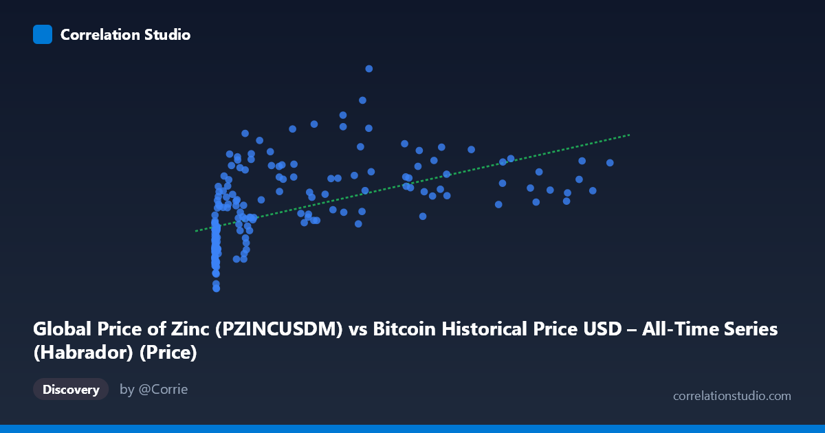
Global Price of Zinc (PZINCUSDM) vs Bitcoin Historical Price USD – All-Time Series (Habrador) (Price)
- Pearson correlation (r)
- 0.5413
- Spearman correlation
- 0.7402
- p-value
- 0
- Sample size (n)
- 189
- 95% confidence interval
- 0.432 to 0.635
- Granger causality
- None
- Granger optimal lag
- 10
- Time coverage
- 2010-08-01 to 2026-04-01
- Recomputed on refreshed data
- 2026-10-06 (r was 0.5351)
AI analysis
Analysis: Bitcoin Price vs. Zinc Price Relationship
1. What the Visualization Reveals
The scatterplot shows a moderate positive relationship between Bitcoin's historical price (X-axis, ranging from fractions of a dollar to $118,670) and global zinc prices (Y-axis, ranging from $1,520 to $4,371/ton). The data reveals a heavily right-skewed X distribution—the vast majority of points cluster below $10,000 (Bitcoin's early-to-mid history), while a smaller number of high-value points extend the range out to six figures. This skew means the visualization is effectively dominated by two distinct regimes: a dense cluster of low-Bitcoin-price/varied-zinc-price points, and a sparser tail of high-Bitcoin-price points that tend to coincide with elevated zinc prices (generally $2,600–$4,000/ton).
2. Strength, Direction, and Statistical Confidence
The Pearson correlation of r = 0.535 indicates a moderate positive linear relationship, with r² = 0.286 meaning only about 28.6% of the variance in zinc prices is explained by Bitcoin price (or vice versa)—leaving over 70% of variance attributable to other factors. The 95% confidence interval [0.425, 0.630] is reasonably tight and entirely positive, and the p-value (2.44×10⁻¹⁵) confirms this correlation is highly statistically significant and not due to chance. However, statistical significance should not be conflated with practical predictive power—r² of 0.29 is modest at best.
Critically, the Granger causality tests show no significant predictive direction in either direction (X→Y: p=0.555; Y→X: p=0.237). This is an important caveat: despite the contemporaneous correlation, neither variable helps forecast the other's future values based on past data. This suggests the relationship is likely driven by a shared external factor (e.g., macroeconomic conditions, USD strength/weakness, global liquidity cycles, or inflation expectations) rather than one asset causally leading the other.
3. Notable Patterns and Non-linear Features
The data is highly non-uniform: for X values under ~1,000, zinc prices vary widely (roughly $1,520–$3,264) with no clear trend, indicating high noise or independent variation during Bitcoin's infancy. As Bitcoin prices climb past $20,000–$40,000, zinc prices increasingly cluster in the $2,800–$4,000 range, suggesting a possible threshold or regime-shift effect rather than a smooth linear scaling. The note that Spearman ρ exceeds Pearson r reinforces this—a monotonic but non-linear relationship (e.g., logarithmic in X, given its extreme scale) likely fits better than the straight line implied by the r² of 0.286. A log-transform of X (Bitcoin price) would probably improve model fit and better reflect Bitcoin's exponential growth pattern.
4. Confounding Factors and Caveats
The most significant caveat is time-series structure: both Bitcoin and zinc prices are non-stationary series with strong trends over 2010–2026, and correlating trending series often produces "spurious" statistical correlation even absent any causal or economic linkage. Both assets may simply be responding to common macro drivers (dollar index, global interest rates, commodity supercycles, industrial demand growth, inflation) rather than influencing each other directly. Additionally, the sampling includes only 188 of 411 total points, and heavy skew in X (mean 20,280 vs. median likely far lower) means outliers/high-leverage points (e.g., the $100,000+ Bitcoin prices) could disproportionately influence the regression slope.
5. Suggestions for Further Investigation
Given the non-stationarity concern, analysts should test both series for unit roots (e.g., ADF test) and consider differencing or examining returns/percentage changes rather than raw price levels to check whether the correlation persists or vanishes (a common outcome with spurious trend-driven correlations). Applying a log transform to Bitcoin price before regression, and exploring partial correlation controlling for a common factor (like DXY dollar index or global M2 money supply), would help clarify whether this is a genuine economic relationship or a shared-trend artifact. Given the lack of Granger causality, this correlation should not be used for predictive trading signals in either direction—it's better framed as a co-movement observation warranting deeper macro-driver analysis rather than a causal or forecasting relationship.
X dataset: Bitcoin Historical Price USD – All-Time Series (Habrador)
Y dataset: Global Price of Zinc
Part of experiment: Bitcoin - Bitcoin Historical Price USD – All-Time Series (Habrador) vs Global Price of Zinc