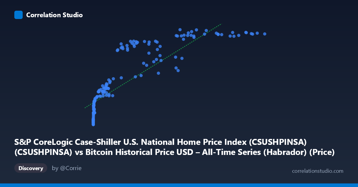
S&P CoreLogic Case-Shiller U.S. National Home Price Index (CSUSHPINSA) (CSUSHPINSA) vs Bitcoin Historical Price USD – All-Time Series (Habrador) (Price)
- Pearson correlation (r)
- 0.8503
- Spearman correlation
- 0.9707
- p-value
- 0
- Sample size (n)
- 189
- 95% confidence interval
- 0.8053 to 0.8856
- Granger causality
- None
- Granger optimal lag
- 9
AI analysis
Analysis: Bitcoin Price vs. Case-Shiller Home Price Index
1. What the Visualization Reveals
This scatterplot juxtaposes Bitcoin's historical USD price (X-axis, spanning from fractions of a cent to $118,670) against the Case-Shiller U.S. National Home Price Index (Y-axis, ranging 134–332). The relationship is strongly monotonic but visibly non-linear: at low Bitcoin values (under ~$100), the home price index clusters tightly in the 135–160 range with very little spread. As Bitcoin climbs into the thousands and tens-of-thousands, Y rises steeply at first, then the curve appears to flatten and even show scatter/reversals at the highest X values (e.g., $56,973 → 278.51 vs. $58,254 → 323.73), suggesting a logarithmic or saturating curve rather than a straight line.
2. Strength, Direction, and Uncertainty
The Pearson r = 0.848 (r² = 0.719) indicates a strong positive linear association, with ~72% of variance in the home price index "explained" by Bitcoin price in a linear model. The 95% CI [0.802, 0.884] is tight and the p-value is effectively zero, meaning the correlation itself is statistically robust — this is not a chance artifact. However, the note that Spearman's ρ exceeds Pearson's r is a strong signal that a monotonic non-linear model (log or power fit) would capture the relationship better than the linear one, consistent with the visual flattening at high X values. Critically, Granger causality tests show no significant predictive direction in either direction (X→Y: p=0.55; Y→X: p=0.58). This means that despite the strong contemporaneous correlation, neither variable's past values meaningfully help forecast the other's future values — the correlation is real but not evidence of temporal lead-lag causality.
3. Notable Patterns and Outliers
The data shows a clear "hockey stick" shape: a long, compressed cluster near the origin (X < $1,000, Y ≈ 135–210) followed by a much more dispersed cloud at higher X values (X $20,000) where Y ranges widely (196–332) for similar X levels — e.g., $41,870→268.71 vs. $44,355→294.90 vs. $45,093→244.17. This heteroscedasticity (variance increasing with X) suggests the relationship weakens or becomes noisier at high Bitcoin valuations, likely because Bitcoin's late-stage volatility (crashes/rallies) is decoupled from the slow-moving, seasonally-driven home price index. The point ($56,973, 278.51) stands out as a local dip amid otherwise higher-Y neighbors, hinting at a Bitcoin crash period overlapping normal home-price growth.
4. Confounding Factors and Caveats
This is almost certainly a spurious or confounded correlation driven by shared trends over time, not a causal economic link. Both series have risen dramatically since 2010–2026: Bitcoin due to adoption/speculation cycles, and home prices due to secular inflation, low interest rates (until 2022), and post-pandemic demand. Any two upward-trending time series will show high correlation without genuine causality — a classic case for spurious regression. The Granger test results confirm this: the correlation is likely an artifact of both variables trending upward over the same 15+ year macroeconomic period (loose monetary policy, inflation, asset-price appreciation broadly) rather than any direct interaction between crypto markets and housing markets.
5. Recommendations for Further Investigation
Given the non-linear hint, refit using a log-transformed X (log(Bitcoin price) vs. Y) or a power/logistic curve, which should substantially improve fit and reduce heteroscedasticity. More importantly, this relationship should be tested with detrended or differenced data (e.g., month-over-month % changes) to check if genuine co-movement exists once the shared upward trend is removed — this is the standard fix for spurious trend-driven correlation. Additionally, consider introducing a common driver variable (e.g., M2 money supply, CPI, or Fed funds rate) as a control to see if it better explains both series jointly, which would confirm this is a shared-macro-driver story rather than a direct Bitcoin-housing relationship.
X dataset: Bitcoin Historical Price USD – All-Time Series (Habrador)
Y dataset: S&P CoreLogic Case-Shiller U.S. National Home Price Index (CSUSHPINSA)
Part of experiment: Bitcoin - Bitcoin Historical Price USD – All-Time Series (Habrador) vs S&P CoreLogic Case-Shiller U.S. National Home Price Index (CSUSHPINSA)