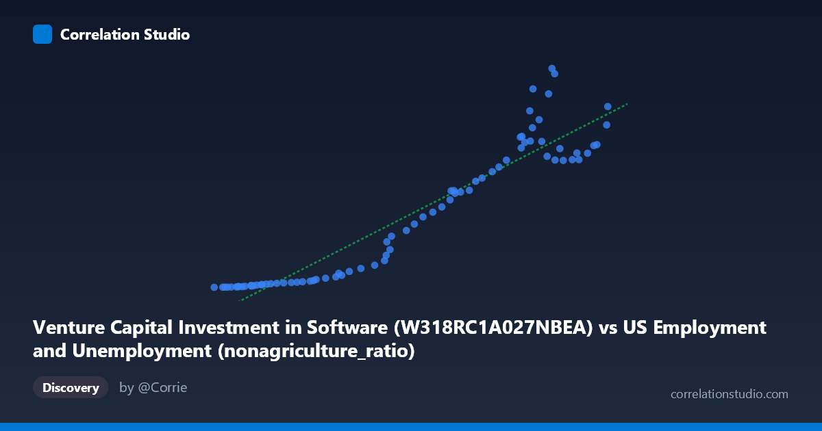
Venture Capital Investment in Software (W318RC1A027NBEA) vs US Employment and Unemployment (nonagriculture_ratio)
- Pearson correlation (r)
- 0.9421
- Spearman correlation
- 0.9595
- p-value
- 0
- Sample size (n)
- 79
- 95% confidence interval
- 0.9108 to 0.9627
- Granger causality
- None
- Granger optimal lag
- 10
AI analysis
Analysis: Venture Capital Investment in Software vs. Non-Agriculture Employment Ratio
Overview of the Relationship
The scatterplot reveals a strong, positive relationship between Venture Capital Investment in Software and the US non-agriculture employment ratio across the 1946–2024 annual time series. As VC investment in software increases, the non-agriculture employment ratio rises in a broadly consistent pattern. The linear regression equation (y = 0.00379568x − 234.238) captures the central tendency well, though the spread of residuals suggests the relationship is not perfectly linear across all value ranges. The data spans a wide X-range (~$46,930M to ~$159,091M), and the corresponding Y-range (0.85 to 466.42) reflects dramatic secular growth in both variables over the study period.
Correlation Strength and Statistical Significance
The Pearson correlation of r = 0.9421 indicates a very strong positive association, and the R² of 0.8876 means that approximately 88.8% of the variance in the non-agriculture employment ratio is statistically explained by VC software investment — a remarkably high figure for socioeconomic data. The 95% confidence interval of [0.9108, 0.9627] is narrow and sits entirely in the high-correlation range, reinforcing the reliability of this estimate with N = 79 paired observations. The p-value of effectively zero confirms this is not a chance finding. However, a critical caveat emerges from the Granger causality analysis: neither direction (X→Y nor Y→X) achieves significance (F = 0.3994, p = 0.9404 and F = 0.5818, p = 0.8206, respectively, at an optimal lag of 10 periods). This means that, despite the strong contemporaneous correlation, neither variable reliably predicts the other temporally, which substantially weakens any causal interpretation.
Patterns, Clusters, and Outliers
The scatterplot shows a clear low-value cluster at the left tail (X < ~75,000; Y < ~25), where the data points are tightly packed and suggest a near-exponential lift-off — small increases in VC investment correspond to disproportionately small employment ratio changes in this regime. In the middle range (~90,000–130,000), data points track the linear fit reasonably well with moderate dispersion. At the upper end (X ~135,000), scatter widens considerably — several notable outliers appear, including (143,194; 466.42), (143,952; 455.02), (137,775; 422.88), and (136,858; 376.19), which sit well above the regression line. Conversely, some high-X points like (146,411; 270.67) and (148,976; 272.29) fall notably below it, suggesting heteroscedasticity and possible non-linearity (perhaps a power or exponential relationship would fit better than OLS linear regression).
Confounding Factors and Interpretive Caveats
The most significant concern is common-trend confounding: both variables are strongly trended over time (reflecting decades of economic growth, technological expansion, and structural labor market shifts), meaning their high correlation may largely reflect shared secular trends rather than a direct functional relationship. This is precisely what the failed Granger causality tests suggest — the two series move together over time but neither drives the other. Additional confounders include macroeconomic cycles (GDP growth, interest rate environments driving both VC activity and employment), the dot-com boom/bust, the 2008 financial crisis, and post-COVID labor market restructuring. The metadata labels also appear swapped or mislabeled (the X-axis is labeled from the "US Employment" dataset but contains what appears to be investment figures, and vice versa), which introduces further interpretive uncertainty and warrants data provenance verification before drawing firm conclusions.
Actionable Insights and Further Investigation
Given the strong correlation but absent Granger causality, the recommended next steps are: (1) Test non-linear model specifications (log-log, power law, or polynomial) given the apparent exponential character of the low-end cluster and the heteroscedasticity at high values; (2) Detrend both series (e.g., first-differencing or HP filter) and re-examine the correlation to isolate cyclical co-movement from shared secular trends; (3) Introduce explicit controls for GDP growth, interest rates, and technology sector share of employment to test whether the bivariate relationship survives in a multivariate framework; (4) Investigate the high-residual outliers (particularly the ~143,000–144,000 X-range cluster) for event-specific explanations (e.g., specific investment boom years); and (5) Resolve the apparent dataset labeling discrepancy before publication or policy use, as axis attribution errors could fundamentally alter the interpretation of directionality.
X dataset: US Employment and Unemployment
Y dataset: Venture Capital Investment in Software
Part of experiment: Yearly - US Employment and Unemployment vs Venture Capital Investment in Software