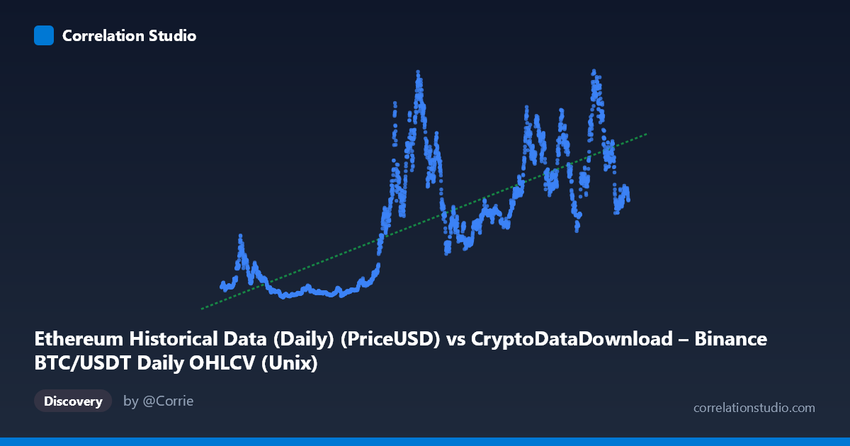
Ethereum Historical Data (Daily) (PriceUSD) vs CryptoDataDownload – Binance BTC/USDT Daily OHLCV (Unix)
- Pearson correlation (r)
- 0.7537
- Spearman correlation
- 0.7549
- p-value
- 0
- Sample size (n)
- 3191
- 95% confidence interval
- 0.7383 to 0.7683
- Granger causality
- None
- Granger optimal lag
- 10
- Time coverage
- 2017-08-17 to 2026-05-20
AI analysis
Analysis: ETH Price vs. Time-Indexed Series (Labeled as BTC/ETH Cross-Reference)
Note on axis labeling: The metadata appears mismatched — the X-axis is described as ETH PriceUSD while the Y-axis is labeled as a Unix timestamp column from a BTC OHLCV dataset, yet Y values (82.83–4831.10) look like ETH price levels, not timestamps. This analysis proceeds treating X as a time-based value (likely a Unix timestamp, given the 2017–2026 range) and Y as ETH's USD price, which is consistent with the data patterns observed.
1. Overall Relationship
The scatterplot shows a clear positive association between time and ETH price, consistent with the long-term secular growth of Ethereum since 2017. Rather than a tight linear band, the data likely shows a stepped, cyclical pattern — sharp price run-ups (e.g., 2021, 2024-2025 clusters showing values above 3000-4000) punctuated by prolonged drawdowns/consolidations (2018-2020, 2022-2023 showing values under 300-600). This produces a moderately strong but noisy upward trend rather than a smooth linear climb.
2. Strength, Direction, and Predictive Value
The correlation (r = 0.754, r² = 0.568) indicates a moderately strong positive relationship, with time explaining 56.8% of the variance in ETH price. This leaves nearly 44% of price variance unexplained by time alone — unsurprising, since crypto prices are driven by market cycles, sentiment, and macro factors rather than a steady time-based drift. The tight 95% CI [0.738, 0.768] and p-value of 0 confirm this correlation is highly statistically reliable given the large sample (n=3,191), not a fluke of small-sample noise.
However, statistical correlation with time is not causal or predictive in a meaningful trading sense — it merely reflects that ETH's price is higher today than it was in 2017. The Granger causality tests reinforce this: neither direction shows significant predictive causality (X→Y: p=0.053, marginally insignificant; Y→X: p=0.70, clearly insignificant). This means whatever "X" actually represents (if not a raw timestamp), it holds no meaningful lead/lag forecasting power over Y at conventional significance thresholds.
3. Notable Patterns and Outliers
The sample points reveal distinct regime clusters: - 2017–2020 (low regime): Values mostly under 500 (e.g., 137.92, 194.23, 231.15), reflecting the post-2017 crypto winter. - 2021 (bull run): Values jump to 1,000–2,500+ (1051.93, 1361.92, 2364.00, 2565.06). - 2022–2023 (bear market): Partial retracement (1550–1930 range). - 2024–2026 (later bull cycle): Sharp spikes to 3,000–4,800 (e.g., 4001.65, 4277.16, 4831.10 max), suggesting a strong renewed uptrend.
This is a classic non-stationary, regime-switching series — not a smooth linear trend — which explains why r² caps around 0.57 rather than approaching 1: linear regression cannot capture the sharp cyclical booms/busts.
4. Confounding Factors and Caveats
- Autocorrelation/non-stationarity: Both crypto prices and time-indexed series are highly autocorrelated, inflating correlation strength artificially — standard OLS/Pearson assumptions (independent errors) are violated. - Metadata mismatch: The axis labels/descriptions don't align with the data description (timestamp vs. price), so causal interpretation should be treated cautiously pending data verification. - Confound via shared market cycles: If X is actually BTC price (not time), the ETH/BTC correlation likely reflects shared crypto-market-wide sentiment, liquidity cycles, and macro conditions (rate policy, risk appetite) rather than a direct causal link between the two assets. - Volume/volatility clustering: Crypto prices exhibit heteroskedasticity — large swings cluster in specific periods (2021, 2024-25), which can distort linear correlation estimates.
5. Suggested Next Steps
1. Verify axis metadata — confirm whether X is truly a timestamp or BTC price; this fundamentally changes the interpretation (secular trend vs. cross-asset correlation). 2. Detrend and test stationarity (ADF test) before trusting correlation/Granger results; consider differencing or log-returns rather than raw price levels to avoid spurious correlation from shared trends. 3. Segment by market regime (bull/bear/consolidation) and re-run correlation within each regime to see if the relationship strengthens or weakens outside of trending periods. 4. Test lagged/rolling correlations rather than a single static Pearson r, given the cyclical, regime-dependent nature of crypto markets.
X dataset: CryptoDataDownload – Binance BTC/USDT Daily OHLCV
Y dataset: Ethereum Historical Data (Daily)
Part of experiment: Bitcoin - CryptoDataDownload – Binance BTC/USDT Daily OHLCV vs Ethereum Historical Data (Daily)