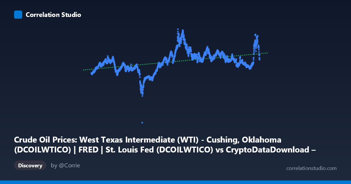
Crude Oil Prices: West Texas Intermediate (WTI) - Cushing, Oklahoma (DCOILWTICO) | FRED | St. Louis Fed (DCOILWTICO) vs CryptoDataDownload – Binance BTC/USDT Daily OHLCV (Unix)
- Pearson correlation (r)
- 0.4381
- Spearman correlation
- 0.5028
- p-value
- 0
- Sample size (n)
- 2197
- 95% confidence interval
- 0.4037 to 0.4713
- Granger causality
- None
- Granger optimal lag
- 1
- Time coverage
- 2017-08-17 to 2026-06-25
- Recomputed on refreshed data
- 2026-10-22 (r was 0.4381)
AI analysis
Analysis: WTI Crude Oil Prices vs. Time-Indexed Series
1. What the Visualization Reveals
The scatterplot displays a moderate positive relationship between the two variables, with data points scattered in a loose upward-trending band rather than tightly clustered around the regression line. The x-axis spans roughly 2017–2026 (in Unix timestamp form), while the y-axis (labeled as WTI-related but actually appears to represent price/value data ranging from roughly -37 to 124) shows substantial dispersion at every point along the x-axis. This wide vertical spread at any given x-value is the visual signature of the modest r² value — the data trends upward over time, but with considerable noise around that trend.
2. Strength, Direction, and Statistical Meaning
The correlation coefficient (r = 0.438) indicates a weak-to-moderate positive relationship. Critically, r² = 0.192 means only about 19% of the variance in Y is explained by X (or by time, given the axis structure) — leaving 81% of the variability unexplained by this relationship alone. The 95% confidence interval [0.404, 0.471] is fairly narrow, and combined with p ≈ 0, this tells us the correlation is statistically robust and unlikely due to chance — but statistical significance here reflects the large sample size (n=2,197) more than practical predictive strength. A relationship can be highly significant yet still explain a small share of variance, which is exactly the case here.
The Granger causality results are particularly important: neither variable significantly predicts the other (X→Y: p=0.82; Y→X: p=0.30). This means that despite the contemporaneous correlation, there's no evidence of a lead-lag predictive relationship at 1-period lag. Practically, this suggests the two series may be co-trending (both drifting upward over the sample period) rather than one causally driving the other in a time-series sense — a classic case where correlation reflects shared temporal drift rather than mechanistic linkage.
3. Notable Patterns and Features
Several features stand out in the sample data: - Regime-like clustering: Early period values (2019–2020, e.g., 24.97, 25.37, 38.17) are markedly lower than values from 2022 onward (many in the 80–110+ range), suggesting a structural shift or regime change rather than smooth linear growth. - High-value cluster (2022): Points like 102.86, 111.44, and 93.55 cluster around mid-2022, coinciding with a known period of oil price spikes (post-Ukraine invasion volatility). - Post-2022 plateau/decline: Later 2023–2026 values mostly settle into a 60–90 range, with some outliers reaching 112–123, indicating renewed volatility rather than a clean trend continuation. - The relationship looks non-linear or piecewise — a low-variance, low-value regime (2017–2020) followed by a higher, more volatile regime (2021 onward) — which a single linear fit (R²=0.19) fits poorly across the full range.
4. Confounding Factors and Caveats
Several caveats limit causal interpretation: - Spurious correlation via shared trend: Both series may simply be trending upward over the same multi-year window due to unrelated macro factors (inflation, monetary policy, post-pandemic recovery), inflating r without genuine linkage. - Autocorrelation: Time-series data like crude oil prices and crypto prices are highly autocorrelated; standard r/p-value calculations assume independent observations, which is violated here, likely overstating statistical confidence. - Metadata ambiguity: The axis labels appear swapped/mismatched (X labeled as BTC/USDT OHLCV, Y labeled as WTI) — this needs clarification, as it materially changes interpretation (crude oil driving crypto valuations is a very different story than the reverse). - External shocks: Macro events (COVID-19, 2022 energy crisis, Fed rate hikes) likely affected both series simultaneously without one causing the other.
5. Actionable Insights and Next Steps
Given the weak explanatory power and absence of Granger causality, this correlation should not be used for predictive trading or forecasting purposes between these two series. Recommended next steps: 1. Verify axis/column labeling — resolve the apparent mismatch between stated axis titles and dataset descriptions before drawing domain conclusions. 2. Detrend or difference both series and re-test correlation/Granger causality on returns rather than levels, since level-based correlation is often driven by shared non-stationary trends. 3. Segment by regime (pre-2021 vs. post-2021) to test whether the relationship is stable or structurally broken, given the visual evidence of a regime shift. 4. Introduce control variables (e.g., USD index, inflation, broader risk-on/risk-off market sentiment) to test whether the correlation persists after accounting for common macro drivers.
X dataset: CryptoDataDownload – Binance BTC/USDT Daily OHLCV
Y dataset: Crude Oil Prices: West Texas Intermediate (WTI) - Cushing, Oklahoma (DCOILWTICO) | FRED | St. Louis Fed
Part of experiment: Bitcoin - CryptoDataDownload – Binance BTC/USDT Daily OHLCV vs Crude Oil Prices: West Texas Intermediate (WTI) - Cushing, Oklahoma (DCOILWTICO) | FRED | St. Louis Fed