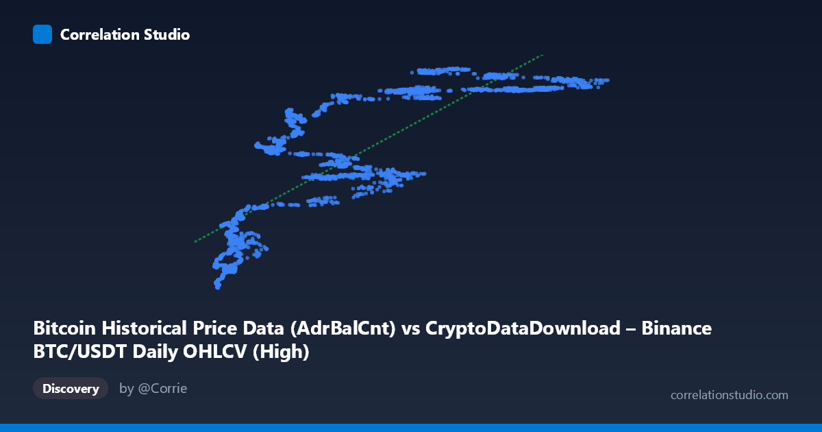
Bitcoin Historical Price Data (AdrBalCnt) vs CryptoDataDownload – Binance BTC/USDT Daily OHLCV (High)
- Pearson correlation (r)
- 0.8282
- Spearman correlation
- 0.8972
- p-value
- 0
- Sample size (n)
- 3191
- 95% confidence interval
- 0.8169 to 0.8388
- Granger causality
- Y → X
- Granger optimal lag
- 10
- Time coverage
- 2017-08-17 to 2026-05-20
AI analysis
Analysis: Bitcoin Active Address Count vs. Price (High)
1. Overall Relationship
The scatterplot depicts a strong positive association between Bitcoin's active address count (AdrBalCnt, X-axis) and its daily high price (Y-axis). As the network's active address count increases from roughly 3,300 to 126,000, the corresponding price high rises from approximately $18.8M to $57M (values appear to be in a scaled/indexed format rather than raw USD). The relationship is broadly monotonic but visibly non-linear — price rises steeply in the low-X range, then shows signs of flattening or plateauing at higher X values, suggesting diminishing marginal price increases per additional active address once the network reaches higher activity levels.
2. Strength, Direction, and Statistical Confidence
The correlation coefficient (r = 0.828) indicates a strong positive linear relationship, with r² = 0.686 meaning roughly 69% of the variance in price highs is statistically explained by variation in active address counts — leaving about 31% attributable to other factors, noise, or non-linear dynamics not captured by this simple linear framework. The 95% confidence interval [0.817, 0.839] is tight, and the p-value of ~0 confirms this correlation is highly unlikely to be due to chance, given the large sample (n=3,191).
Importantly, the Granger causality results complicate a naive "more addresses drive price" narrative: the test found Y Granger-causes X (price predicts future active address counts), not the reverse (X→Y was not significant at p=0.149, while Y→X was significant at p=0.041). This suggests that price movements may be leading indicators of network activity — plausibly because price rallies attract new users/wallets — rather than address growth driving price appreciation. This is a meaningful reframing: correlation strength alone would tempt an "adoption drives price" story, but the temporal evidence points the other way.
3. Patterns, Clusters, and Outliers
Several structural patterns are visible in the sampled data: - Low-X cluster (X < 15,000): Prices are tightly clustered in the $19M–$33M range with a fairly steep slope, suggesting this region behaves almost like a distinct regime. - Mid-range scatter (X: 20,000–60,000): Notable heteroskedasticity — for similar X values (e.g., ~25,000–30,000), Y ranges from $33M to $49M, indicating other factors modulate price beyond address count alone. - High-X plateau (X 60,000): Prices compress into a narrower $51M–$57M band despite X ranging up to 126,000, reinforcing the impression of saturation/diminishing returns at high network activity. - No extreme outliers are apparent, but the compression at both tails suggests the true relationship may be better modeled as logarithmic or S-curved rather than strictly linear.
4. Confounding Factors and Caveats
Several caveats limit causal interpretation: - Time-series autocorrelation: Both series are trending over an 8+ year span (2017–2026) and likely share common macro drivers (bull/bear cycles, halving events, regulatory shifts, exchange volume trends) that could inflate correlation without direct causal linkage. - Address count is a noisy proxy: AdrBalCnt can be inflated by exchange-internal address churn, wallet-splitting behavior, or dust transactions, decoupling it from genuine user adoption. - Non-stationarity: Price and on-chain metrics are both non-stationary series; a Granger test on levels (rather than differenced/detrended data) can produce spurious directional signals if not properly controlled for. - Scale/units ambiguity: The Y-axis values (tens of millions) don't match typical BTC/USDT price scales, suggesting some aggregation, indexing, or currency conversion — this should be clarified before drawing price-specific conclusions.
5. Suggested Next Steps
1. Re-run Granger causality on differenced/log-transformed and detrended series to rule out spurious correlation from shared trends and confirm the Y→X directionality holds after removing non-stationarity. 2. Fit non-linear models (log-log, logistic, or piecewise regression) to better capture the apparent saturation effect at high address counts. 3. Segment by market regime (bull vs. bear, halving cycles) to check if the r² and slope are stable or regime-dependent. 4. Incorporate additional on-chain controls (transaction volume, exchange inflows/outflows, hash rate) to isolate the address-count effect from other confounds. 5. Validate the Y-axis units/definition with the data source before using this model for price forecasting, given the unusually large scale relative to known BTC/USDT price history.
X dataset: CryptoDataDownload – Binance BTC/USDT Daily OHLCV
Y dataset: Bitcoin Historical Price Data
Part of experiment: Bitcoin - CryptoDataDownload – Binance BTC/USDT Daily OHLCV vs Bitcoin Historical Price Data