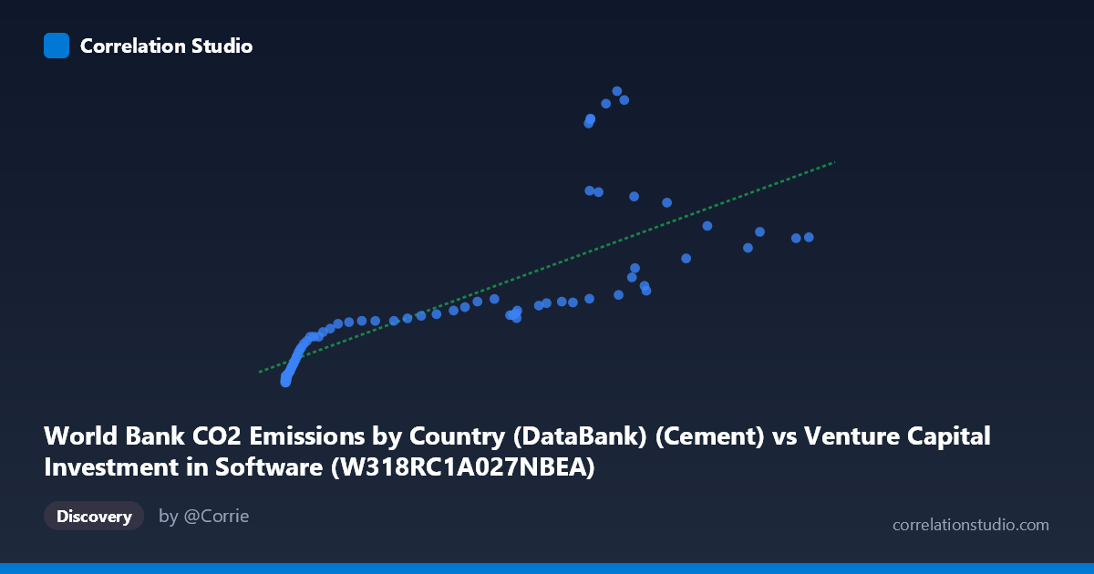
World Bank CO2 Emissions by Country (DataBank) (Cement) vs Venture Capital Investment in Software (W318RC1A027NBEA)
- Pearson correlation (r)
- 0.7709
- Spearman correlation
- 0.9594
- p-value
- 0
- Sample size (n)
- 75
- 95% confidence interval
- 0.6593 to 0.8493
- Granger causality
- None
- Granger optimal lag
- 10
- Time coverage
- 1946-01-01 to 2020-01-01
- Recomputed on refreshed data
- 2026-10-24 (r was 0.7709)
AI analysis
Scatterplot Analysis: Cement CO2 Emissions vs. Venture Capital Investment in Software
1. Overall Relationship
The scatterplot reveals a positive association between World Bank CO2 emissions from cement production and venture capital investment in software, spanning annual data from 1946 to 2020. As cement CO2 emissions increase, software VC investment tends to rise as well. However, the relationship is clearly not uniformly linear — the data exhibits two visually distinct behavioral zones: a dense cluster of points at lower X values (below ~150) where Y rises steeply and variably, and a more dispersed middle range (150–470) where the relationship flattens and becomes noisier. This bifurcated structure immediately signals that a single linear model may be an oversimplification.
2. Correlation Strength, Direction, and Causality
The Pearson correlation of r = 0.7709 indicates a moderately strong positive relationship, and the p-value of 6.661×10⁻¹⁶ confirms this is extraordinarily unlikely to be due to chance alone. However, the R² of 0.5942 is the more sobering metric — it means that roughly 59.4% of variance in VC software investment is explained by cement CO2 emissions, leaving over 40% unaccounted for by this model. The 95% confidence interval for r of [0.6593, 0.8493] is reasonably tight, suggesting the estimate is stable, though the upper and lower bounds still span a meaningful range of practical effect sizes. Critically, the Granger causality results show no significant predictive directionality in either direction (X→Y: F=0.533, p=0.857; Y→X: F=1.314, p=0.253), meaning that past values of cement emissions do not help predict future VC investment, and vice versa. This strongly implies the correlation reflects shared temporal trends or a common driving force rather than any meaningful causal mechanism between these two specific variables.
3. Notable Patterns, Clusters, and Outliers
Several features stand out on close inspection:
- High-leverage outliers at mid-range X (~270–310): A cluster of points around X = 270–310 shows dramatically elevated Y values (1,746–2,608), well above the regression line. These points — including (295.91, 2608.93), (302.31, 2532.94), (286.07, 2501.79), and (272.29, 2374.89) — likely correspond to the late 1990s dot-com investment surge, when VC in software exploded independently of cement trends. - Steep curvature at low X values (0–50): Points with X < 50 show Y values ranging from ~121 to ~582, a spread that is disproportionately wide relative to that X range. This steep initial rise is consistent with a logarithmic or power-law relationship, which explains why Spearman ρ exceeds Pearson r — rank-based correlation captures this non-linear ascent better. - Plateau behavior at higher X (150–466): Above X ≈ 150, Y values spread broadly between ~670 and ~1,361 with no strong slope, suggesting diminishing marginal association and possible regime change in the underlying dynamics. - The point (1.53, 121.42) appears to be the minimum anchor, likely representing early postwar years when both cement production and VC activity were negligible.
4. Confounding Factors and Interpretive Caveats
The most important caveat here is that this correlation almost certainly reflects a shared dependence on time and global economic growth rather than any substantive link between cement emissions and software investment. Both variables trend upward over the 1946–2020 period as industrialization and technological investment both expanded — this is a textbook case of spurious correlation driven by secular trends. The column labeling in the dataset metadata also appears inverted (cement CO2 data is labeled under a VC dataset and vice versa), which raises data provenance concerns that should be verified before drawing any conclusions. Additionally, the optimal Granger lag of 10 periods is quite long, and the non-significant result across all lags further reinforces that temporal structure does not support a predictive relationship. The non-linearity flagged by the Spearman/Pearson divergence means the linear regression equation (y = 3.50x + 289.5) systematically underestimates Y at low and high X values while overestimating it in the middle range.
5. Actionable Insights and Further Investigation
Given these findings, the following steps would strengthen the analysis:
- Detrend both series (e.g., first-differencing or removing a time trend) before recomputing correlation, to test whether the relationship holds beyond shared temporal growth trajectories. - Fit a logarithmic or polynomial model — the non-linear signal is strong enough (Spearman Pearson) to warrant comparing AIC/BIC across model families; a log(X) transformation of cement emissions may substantially improve fit. - Investigate the outlier cluster (X ≈ 270–310, Y 1,700) by mapping these points to specific years — they likely correspond to the 1998–2001 dot-com boom, and treating this as a structural break or dummy variable could improve model stability. - Introduce GDP or year as a covariate in a multivariate model to partial out the confounding effect of shared economic time trends. - Verify dataset column assignment, as the metadata descriptions appear switched between X and Y axes, which could fundamentally alter the interpretation of the entire analysis.
X dataset: Venture Capital Investment in Software
Y dataset: World Bank CO2 Emissions by Country (DataBank)
Part of experiment: Yearly - Venture Capital Investment in Software vs World Bank CO2 Emissions by Country (DataBank)