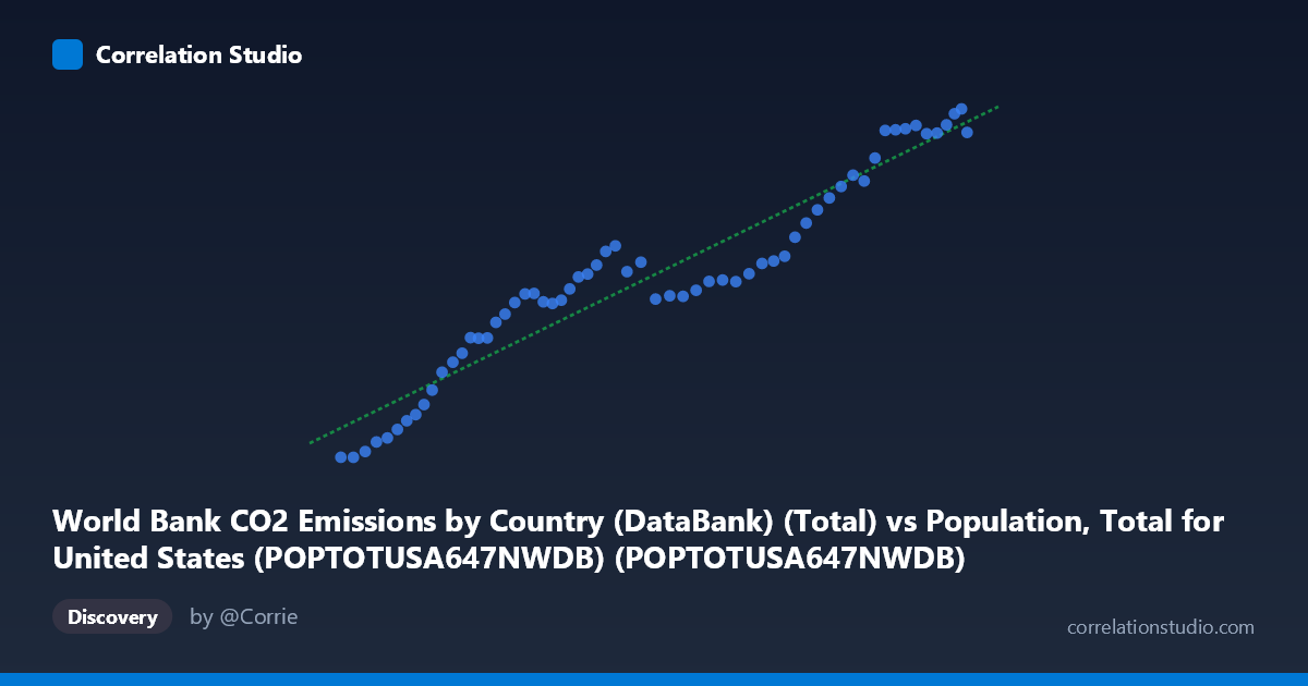
World Bank CO2 Emissions by Country (DataBank) (Total) vs Population, Total for United States (POPTOTUSA647NWDB) (POPTOTUSA647NWDB)
- Pearson correlation (r)
- 0.955
- Spearman correlation
- 0.9632
- p-value
- 0
- Sample size (n)
- 61
- 95% confidence interval
- 0.9259 to 0.9729
- Granger causality
- None
- Granger optimal lag
- 10
AI analysis
Analysis: U.S. Population vs. CO₂ Emissions (1960–2020)
1. Overall Relationship The scatterplot reveals a strong, positive relationship between total U.S. population and CO₂ fossil fuel emissions over the 1960–2020 period. As population grows, CO₂ emissions rise in a broadly consistent pattern, with the data points tracking closely along the fitted regression line (y = 0.000171x − 14,716). The visual impression is one of a tight, upward-sweeping arc with relatively little scatter around the central trend, suggesting that population size is a powerful co-variate of national emissions across this six-decade window.
2. Correlation Strength and Statistical Interpretation The Pearson correlation of r = 0.9550 is exceptionally strong, and the coefficient of determination r² = 0.9121 indicates that approximately 91.2% of the variance in CO₂ emissions is statistically explained by U.S. population size in this sample. The 95% confidence interval for r [0.9259, 0.9729] is notably narrow, confirming that this is not a fragile estimate — the true population correlation is almost certainly very high. The p-value of effectively 0 (against n = 61 paired observations) rules out chance as an explanation for the association. However, the Granger causality tests complicate any causal narrative: neither direction (X→Y: F = 1.25, p = 0.30; Y→X: F = 1.31, p = 0.27) achieves statistical significance at conventional thresholds, even with an optimal lag of 10 periods. This means that, in a strictly temporal predictive sense, knowing past population values does not significantly improve forecasts of future emissions beyond what emissions history alone provides, and vice versa. The correlation is real and robust, but the causal arrow is statistically indeterminate from this analysis alone.
3. Notable Patterns, Clusters, and Features Visually, the data appear to follow a slightly sigmoidal or mildly non-linear trajectory rather than a perfectly straight line. Points in the lower-left cluster (population ~180–210 million, emissions ~13,700–22,500 kt, roughly 1960s–early 1970s) rise steeply, suggesting rapid emissions growth per capita during early industrialization of that era. The middle range (population ~230–270 million, emissions ~26,000–31,000 kt, roughly mid-1970s to early 1990s) shows a noticeably flatter slope and increased horizontal scatter — consistent with post-oil-crisis efficiency gains and emissions plateauing despite continued population growth. The upper-right cluster (population ~295–331 million, emissions ~33,000–43,000 kt, roughly 2000s–2020) resumes a steeper incline. This structural break in slope is an important feature that a single linear model partially obscures, and it hints that the emissions-per-person relationship changed substantially over time.
4. Confounding Factors and Caveats The most important caveat is that population and time are deeply collinear in this dataset — both increase monotonically over the same 60-year window, meaning the correlation may largely reflect shared temporal trending rather than a direct mechanistic link between headcount and emissions. Genuine drivers of emissions — GDP growth, energy mix transitions, industrial structure shifts, fuel efficiency regulations, offshoring of manufacturing, and policy interventions (e.g., Clean Air Act amendments, the shale gas transition displacing coal) — are all omitted from this bivariate framing. The apparent flattening in the mid-range is almost certainly attributable to these factors rather than population dynamics per se. Additionally, the dataset covers only the U.S., so findings should not be generalized globally without accounting for vastly different development trajectories elsewhere. The high r² should therefore be interpreted as reflecting covariation across time, not a clean causal pathway from population to emissions.
5. Actionable Insights and Further Investigation Given the structural break in slope visible in the mid-range, a piecewise regression or segmented analysis (pre-/post-1973 oil shock; pre-/post-2005 shale transition) would better capture the true relationship dynamics. Incorporating per-capita emissions as a derived variable and regressing it against time, GDP per capita, or energy intensity would help isolate whether population growth is genuinely driving emissions or simply serving as a proxy for economic expansion. Granger causality tests with shorter lag structures or using first-differenced (growth rate) data rather than levels would reduce the influence of shared trend and provide a cleaner test of temporal predictability. Finally, multivariate panel analysis — extending to multiple countries with varying population growth rates and emissions trajectories — would be the most robust way to determine whether the population–emissions relationship is structurally stable or an artifact of U.S.-specific historical co-trending.
X dataset: Population, Total for United States (POPTOTUSA647NWDB)
Y dataset: World Bank CO2 Emissions by Country (DataBank)
Part of experiment: Yearly - Population, Total for United States (POPTOTUSA647NWDB) vs World Bank CO2 Emissions by Country (DataBank)