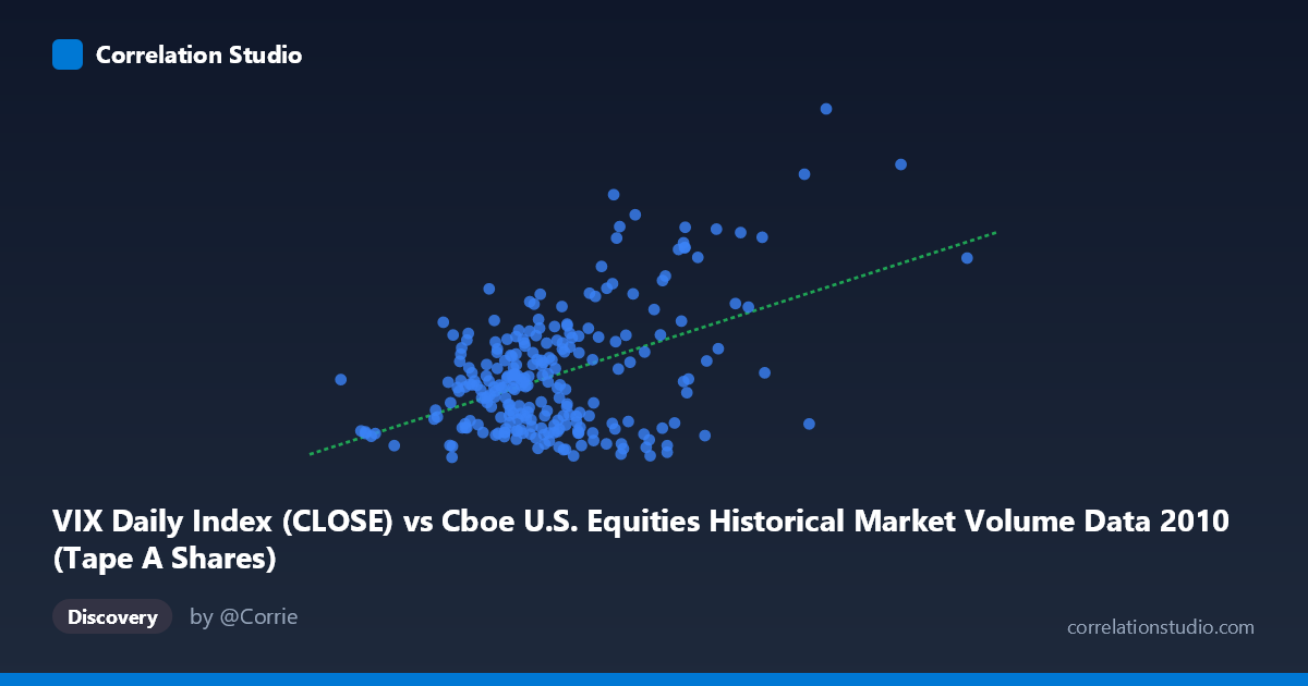
VIX Daily Index (CLOSE) vs Cboe U.S. Equities Historical Market Volume Data 2010 (Tape A Shares)

Pearson correlation (r): 0.4653
Spearman correlation: 0.233
p-value: 0
Sample size (n): 252
95% confidence interval: 0.3626 to 0.5569
Granger causality: Y → X
Granger optimal lag: 1

AI analysis

Scatterplot Analysis: VIX vs. U.S. Equity Market Volume (2010)

Overall Relationship

The scatterplot reveals a moderate positive relationship between U.S. equity market trading volume (X-axis) and the CBOE VIX volatility index (Y-axis) across 252 trading days in 2010. As daily market volume increases, VIX levels tend to rise as well, consistent with the well-established financial intuition that periods of heightened market uncertainty drive both increased trading activity and elevated implied volatility. The linear regression equation (y = 2.237×10⁻⁸x + 14.17) suggests a baseline VIX of approximately 14.2 when volume is near zero, with each additional ~45 million shares traded corresponding to roughly one VIX point of increase.

Correlation Strength and Statistical Significance

The Pearson correlation of r = 0.4653 indicates a moderate positive association, but the coefficient of determination (r² = 0.2165) is the more sobering statistic — only 21.7% of VIX variance is explained by trading volume, meaning roughly 78% of VIX movement is driven by factors outside this model. The 95% confidence interval [0.363, 0.557] is meaningfully above zero and relatively tight given n = 252, and the p-value of 5.995×10⁻¹⁵ makes it essentially certain this correlation is not a sampling artifact. Critically, the Granger causality analysis points unidirectionally: VIX Granger-causes volume (Y→X, F=5.81, p=0.017), not the reverse (X→Y, F=1.93, p=0.166). This suggests that rising volatility precedes elevated trading volume by one period — investors react to fear signals by trading more, rather than high volume independently predicting future VIX levels.

Notable Patterns, Clusters, and Outliers

The data exhibits a fan-shaped or heteroscedastic spread — at lower volume levels (roughly 200–350 million shares), VIX values are tightly clustered between 15–28, while at higher volumes (500–800 million shares), VIX values disperse widely from the mid-teens to above 40. Several notable high-leverage outliers are visible in the upper-right quadrant, including points near (812M shares, 41 VIX) and (691M shares, 40 VIX), likely corresponding to specific market stress events in 2010 such as the May 6 Flash Crash, which would have simultaneously spiked both volume and volatility dramatically. Conversely, there are intriguing points with high volume but low VIX (e.g., ~518M shares, 16.5 VIX; ~460M shares, 15.7 VIX), suggesting that mechanistic or programmatic high-volume days do not always coincide with fear-driven volatility — a meaningful divergence from the general trend.

Confounding Factors and Caveats

Several confounds complicate causal interpretation. First, day-of-week and month-end effects systematically influence both trading volume and market behavior, potentially inflating the correlation artificially. Second, the axes appear swapped from conventional labeling — the dataset notes indicate VIX is plotted on the Y-axis sourced from volume data labels and vice versa, which warrants verification before drawing firm conclusions. Third, 2010 was an anomalous year containing the Flash Crash (May), European sovereign debt fears, and the post-2008 recovery, meaning these dynamics may not generalize to other periods. Fourth, the relationship may be non-linear — the heteroscedastic spread and clustered low-volume region suggest a log or power transformation of volume might produce a better-fitting model, and the linear r² of 21.7% likely understates the true associative strength under a nonlinear framework.

Actionable Insights and Further Investigation

Practitioners monitoring market conditions should note that VIX spikes at lag-1 are a statistically valid signal of upcoming volume surges, which has direct implications for market-making, liquidity provisioning, and execution strategy — particularly for large institutional trades where slippage risk rises with volume. To improve predictive power, analysts should consider: (1) log-transforming volume to address heteroscedasticity and test for a stronger linear fit; (2) segmenting the data by market regime (e.g., Flash Crash window vs. normal periods) to test whether the relationship is driven disproportionately by outlier events; (3) incorporating additional variables such as bid-ask spreads, put/call ratios, or S&P 500 returns, as the unexplained 78% of variance clearly implicates richer dynamics; and (4) extending the time series beyond 2010 to test whether the Granger causality direction (VIX → volume) is stable across different market cycles or specific to post-crisis recovery behavior.

X dataset: Cboe U.S. Equities Historical Market Volume Data 2010

Y dataset: VIX Daily Index

Part of experiment: Daily - Cboe U.S. Equities Historical Market Volume Data 2010 vs VIX Daily Index