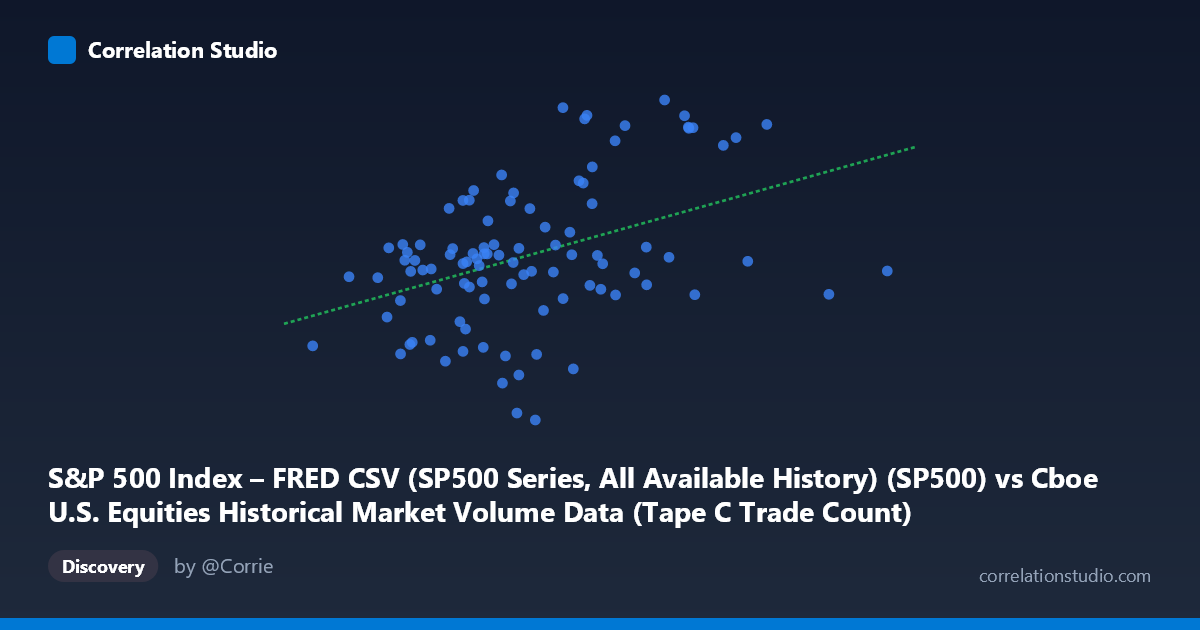
S&P 500 Index – FRED CSV (SP500 Series, All Available History) (SP500) vs Cboe U.S. Equities Historical Market Volume Data (Tape C Trade Count)
- Pearson correlation (r)
- 0.4154
- Spearman correlation
- 0.347
- p-value
- 0.000021
- Sample size (n)
- 98
- 95% confidence interval
- 0.2364 to 0.567
- Granger causality
- None
- Granger optimal lag
- 10
AI analysis
Scatterplot Analysis: S&P 500 Index vs. Cboe Tape C Trade Count
Relationship Overview
The scatterplot reveals a modest positive relationship between the S&P 500 Index level (X-axis, ranging approximately 2.58M–4.34M in the dataset's scaled units) and Cboe U.S. Equities Tape C Trade Count (Y-axis, ranging from ~6,344 to ~7,501). As the S&P 500 rises, Tape C trade counts tend to drift upward as well, consistent with the intuition that bull market environments attract greater retail and institutional participation in exchange-listed securities. However, the scatter is notably wide, with substantial vertical dispersion at nearly every X-value, indicating that the index level alone is far from a reliable predictor of daily trade activity.
Correlation Strength and Statistical Interpretation
The Pearson correlation of r = 0.4154 reflects a weak-to-moderate positive association. More telling is the r² = 0.1725, meaning the S&P 500 level explains only ~17.3% of the variance in Tape C trade counts — leaving roughly 82.7% of variation unexplained by this relationship alone. The linear regression equation (y = 0.000330x + 5868.82) confirms a very shallow slope, implying that even large moves in the index translate into relatively small predicted changes in trade count. The 95% confidence interval for r of [0.2364, 0.5670] is meaningfully wide, reflecting genuine uncertainty around the true population correlation, though the interval excludes zero. The p-value of 2.111×10⁻⁵ confirms the correlation is statistically significant at conventional thresholds given n = 98, so the relationship is unlikely to be a sampling artifact. Critically, however, the Granger causality tests show no significant predictive directionality in either direction (X→Y: F = 0.66, p = 0.757; Y→X: F = 1.10, p = 0.373), even at the optimal lag of 10 periods. This means neither variable reliably predicts future movements in the other in a temporal sense — the correlation is contemporaneous at best, not mechanically causal.
Patterns, Clusters, and Outliers
Several structural features are visible in the data. There appears to be a loose cluster of observations in the X range of ~2.9M–3.5M with Y values concentrated between ~6,600–7,100, forming the dense core of the scatter. At higher S&P 500 levels (X 3.6M), points tend to shift toward higher Y values (7,300–7,500), supporting the positive trend, but the sample thins considerably, reducing confidence in that region. A few notable outliers are evident: one point near (3,262,293, 6,344) sits well below the regression line, representing an unusually low Tape C trade count despite a mid-range index level; similarly, (3,205,940, 6,369) and (3,161,454, 6,477) appear as low-trade-count anomalies. On the upper end, (3,658,891, 7,501) and (3,347,013, 7,473) represent high-activity sessions. These extremes may correspond to specific market events (volatility spikes, holidays, or structural market disruptions) rather than reflecting the general trend.
Confounding Factors and Interpretive Caveats
Several important caveats apply. First, the dataset labels appear to be swapped or mislabeled — the X-axis is described as "S&P 500 Index" from a Cboe volume dataset, and the Y-axis as "Tape C Trade Count" from a FRED S&P 500 dataset, which suggests a possible data pipeline or column assignment error that should be verified before drawing firm conclusions. Second, Tape C trade count is influenced by factors entirely independent of index level: market microstructure changes, exchange rule updates, seasonal trading patterns, macroeconomic announcements, and the rise of algorithmic trading all affect daily trade counts. Third, the time window (Jan–May 2026) is narrow, covering only ~5 months, which limits generalizability and may capture a regime-specific relationship that doesn't hold across full market cycles. Fourth, the N = 1,980 population figure versus n = 98 sample suggests significant undersampling, and results could shift with a fuller dataset.
Actionable Insights and Further Investigation
Given the modest explanatory power and absent Granger causality, practitioners should not use S&P 500 levels alone as a signal for Tape C trading activity. Instead, the following steps are recommended: (1) Verify column assignments and data provenance to rule out a labeling error; (2) Incorporate additional predictors — such as VIX (implied volatility), market breadth indicators, or time-of-year seasonality — into a multivariate model to better explain trade count variance; (3) Extend the time series to the full available history to test whether this relationship is stable across different market regimes (e.g., bear markets, post-pandemic periods); (4) Investigate the low-trade-count outliers individually to determine if they represent data quality issues or economically meaningful events; and (5) Test non-linear specifications (e.g., quadratic or piecewise regression), as the scatter hints at possible threshold effects at higher index levels where trade counts cluster at elevated values.
X dataset: Cboe U.S. Equities Historical Market Volume Data
Y dataset: S&P 500 Index – FRED CSV (SP500 Series, All Available History)
Part of experiment: Daily - Cboe U.S. Equities Historical Market Volume Data vs S&P 500 Index – FRED CSV (SP500 Series, All Available History)