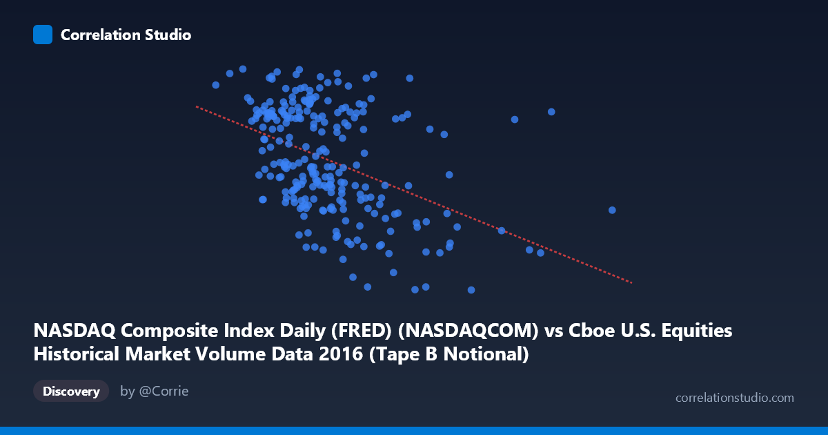
NASDAQ Composite Index Daily (FRED) (NASDAQCOM) vs Cboe U.S. Equities Historical Market Volume Data 2016 (Tape B Notional)
- Pearson correlation (r)
- -0.4361
- Spearman correlation
- -0.4421
- p-value
- 0
- Sample size (n)
- 252
- 95% confidence interval
- -0.5311 to -0.3304
- Granger causality
- None
- Granger optimal lag
- 10
- Time coverage
- 2016-01-04 to 2016-12-30
- Recomputed on refreshed data
- 2026-10-24 (r was -0.4361)
AI analysis
Scatterplot Analysis: NASDAQ Composite Index vs. Cboe Tape B Notional Volume (2016)
Overall Relationship
The scatterplot reveals a negative relationship between the NASDAQ Composite Index daily closing values (X-axis) and Cboe U.S. Equities Tape B notional trading volume (Y-axis) across 252 trading days in 2016. As the NASDAQ index climbs higher — particularly in the upper range above ~7–8 billion — notional volume tends to decline, while lower index values cluster around higher notional figures. The linear regression equation (y = −8.30×10⁻⁸x + 5406.7) confirms this inverse slope, though the visual spread around the regression line is substantial, suggesting the relationship is real but far from deterministic.
Correlation Strength and Statistical Significance
The Pearson correlation of r = −0.4361 indicates a moderate negative association. However, r² = 0.1902 means that only about 19% of the variance in Tape B notional volume is explained by the NASDAQ index level — leaving roughly 81% attributable to other factors. While this is statistically significant (p = 4.0×10⁻¹³, effectively zero), the 95% confidence interval of [−0.5311, −0.3304] confirms the effect is reliably negative but modest in magnitude. Crucially, the Granger causality tests show no significant directional predictive relationship in either direction (X→Y: F = 0.19, p = 0.997; Y→X: F = 0.49, p = 0.894), meaning that knowing today's NASDAQ level does not help predict tomorrow's Tape B volume, and vice versa. Correlation here reflects a contemporaneous association, not a temporal leading/lagging dynamic.
Notable Patterns, Clusters, and Outliers
Several structural features stand out in the data. The bulk of observations cluster between ~3.5–6.0 billion on the X-axis and 4,700–5,400 on the Y-axis, forming a moderately dense central cloud with a visible downward drift. There appear to be notable outliers at higher X values — points near 8.0–12.7 billion in NASDAQ volume that sit at relatively low Tape B notional values (~4,400–4,600), pulling the regression line and potentially inflating the negative correlation. The sample points confirm this: (8,200,813,716, 5,125.91) and (8,084,440,928, 4,472.06) represent divergent behavior at high-X values, suggesting non-linear or regime-based dynamics. There may also be a mild non-linear (curved) structure in the data — the relationship may be steeper at extreme X values than in the central cluster.
Confounding Factors and Caveats
Several important caveats apply to this interpretation. First, both variables are time-indexed to 2016, meaning shared temporal trends (e.g., post-Brexit volatility spikes in mid-2016, the U.S. election in November) could be driving both series independently, producing a spurious or context-dependent correlation. High-volatility events often simultaneously depress index levels and spike notional volumes, which mechanically generates the observed negative pattern. Second, Tape B notional volume covers a specific subset of exchanges (non-NYSE, non-NASDAQ-listed securities traded on other venues), which may not be the most natural counterpart to the NASDAQ Composite. Third, the population size (N = 3,622) is notably larger than the sample (n = 252), suggesting the full dataset may yield somewhat different estimates. Finally, the lack of Granger causality at a 10-period lag should not be interpreted as absence of any causal mechanism — lagged effects at other horizons were not tested.
Actionable Insights and Further Investigation
Despite the modest explanatory power, this negative relationship carries practical implications for market microstructure analysis. Rising index levels in 2016 may reflect calmer, trending markets where less rebalancing and hedging activity drives Tape B venue volume down, while falling markets drive defensive trading flows. To deepen the analysis, investigators should: (1) test for non-linear or regime-switching models (e.g., segmenting by high/low volatility regimes using VIX data); (2) include intraday volatility or VIX as a covariate to test whether it mediates or confounds the relationship; (3) expand Granger causality testing to shorter lags (1–5 periods) and broader lag ranges to rule out short-term predictive dynamics; and (4) compare Tape A and Tape C notional volumes against the same index to assess whether this pattern is venue-specific or systemic across U.S. equity market structure.
X dataset: Cboe U.S. Equities Historical Market Volume Data 2016
Y dataset: NASDAQ Composite Index Daily (FRED)
Part of experiment: Daily - Cboe U.S. Equities Historical Market Volume Data 2016 vs NASDAQ Composite Index Daily (FRED)