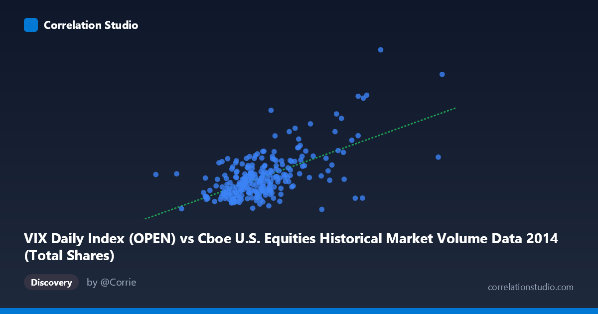
VIX Daily Index (OPEN) vs Cboe U.S. Equities Historical Market Volume Data 2014 (Total Shares)
- Pearson correlation (r)
- 0.6096
- Spearman correlation
- 0.498
- p-value
- 0
- Sample size (n)
- 252
- 95% confidence interval
- 0.5256 to 0.6818
- Granger causality
- None
- Granger optimal lag
- 1
AI analysis
Analysis: VIX Daily Index vs. U.S. Equities Market Volume (2014)
Relationship Overview The scatterplot reveals a positive relationship between U.S. equities market trading volume (X-axis) and the VIX Daily Index open values (Y-axis) across 252 trading days in 2014. As total shares traded increases, VIX levels tend to rise, which aligns intuitively with the well-established market dynamic that elevated volatility accompanies heightened trading activity. Periods of fear or uncertainty drive investors to trade more actively while simultaneously pushing the VIX higher. The linear regression equation (y = 1.84×10⁻⁸x + 6.15) indicates a very small per-unit slope, reflecting the vast scale difference between share counts (hundreds of millions) and VIX values (roughly 10–30).
Correlation Strength and Statistical Significance The Pearson correlation of r = 0.6096 indicates a moderate-to-strong positive association, but the explanatory power is more modest: r² = 0.3716 means only ~37.2% of the variance in VIX is explained by trading volume, leaving nearly 63% attributable to other factors. The 95% confidence interval of [0.526, 0.682] is reasonably tight given a sample of 252, and the p-value of effectively zero confirms this is not a chance finding across the N = 3,686 population context. However, Granger causality tests reveal no significant temporal predictive direction in either direction — neither X→Y (F = 0.79, p = 0.37) nor Y→X (F = 0.18, p = 0.68) — meaning that while the two variables move together contemporaneously, past values of volume do not reliably predict future VIX, and vice versa. This critically distinguishes correlation from predictive utility and cautions against using one variable as a leading indicator for the other.
Notable Patterns, Clusters, and Outliers The data exhibits several visually distinct features worth noting: - A dense core cluster sits between approximately 350–500 million shares and VIX values of 11–17, representing the "normal" trading environment for most of 2014, when markets were relatively calm - A sparse high-volume, high-VIX tail extends toward the upper right, with notable outliers around (670M shares, 23.6) and one extreme point near (710M shares, 29.3) — likely corresponding to specific volatility events such as the October 2014 market correction driven by Ebola fears and global growth concerns - A curious low-VIX, high-volume point near (575M shares, 10.4) breaks the general trend, suggesting volume can surge without corresponding fear — possibly index rebalancing or options expiration activity - The lower-left region (sub-300M shares, VIX ~11–15) shows a distinct secondary cluster, possibly reflecting early-year low-activity periods
Confounding Factors and Caveats Several important caveats temper interpretation. Simultaneity bias is a concern — VIX and volume are likely jointly determined by underlying market events (geopolitical shocks, Fed announcements, earnings seasons) rather than one causing the other, which the failed Granger tests support. Seasonality is a significant confounder: both trading volume and volatility follow known calendar patterns (e.g., August/December lulls, October spikes), so the correlation may partly reflect shared seasonal rhythms rather than a direct economic link. Additionally, the dataset and variable labeling appear inverted in the axis descriptions (the dataset name suggests X contains VIX data while Y contains volume data from the Cboe dataset), which warrants verification before drawing directional conclusions. Finally, 2014 was a broadly low-volatility year punctuated by isolated spikes, so results may not generalize to other market regimes.
Actionable Insights and Further Investigation Practitioners and researchers should consider the following next steps: 1. Control for known event dates (FOMC meetings, options expirations, the October 2014 correction) using dummy variables to isolate the "pure" volume-volatility relationship 2. Test non-linear specifications — a logarithmic or power-law model may better capture the apparent heteroscedasticity where variance fans out at higher volume levels 3. Extend the time series across multiple years (2008–2024) to test whether this r ≈ 0.61 relationship is stable across different volatility regimes or breaks down in crisis periods 4. Incorporate intraday data to examine whether the relationship strengthens at finer time resolutions, where mechanical links between volume and realized volatility are well-documented 5. Investigate the outlier cluster (October 2014 specifically) as a natural experiment to understand what drives departure from the central tendency
X dataset: Cboe U.S. Equities Historical Market Volume Data 2014
Y dataset: VIX Daily Index
Part of experiment: Daily - Cboe U.S. Equities Historical Market Volume Data 2014 vs VIX Daily Index