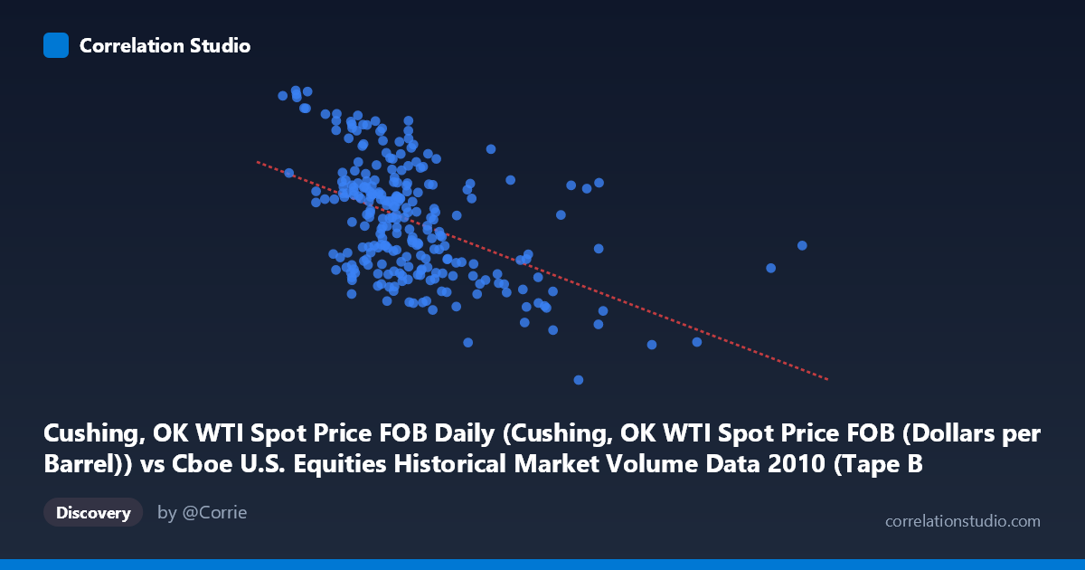
Cushing, OK WTI Spot Price FOB Daily (Cushing, OK WTI Spot Price FOB (Dollars per Barrel)) vs Cboe U.S. Equities Historical Market Volume Data 2010 (Tape B Notional)
- Pearson correlation (r)
- -0.4909
- Spearman correlation
- -0.475
- p-value
- 0
- Sample size (n)
- 252
- 95% confidence interval
- -0.5793 to -0.391
- Granger causality
- None
- Granger optimal lag
- 1
AI analysis
Analysis: WTI Crude Oil Price vs. Cboe Tape B Notional Value (2010)
Relationship Overview
The scatterplot reveals a moderate negative relationship between WTI crude oil spot prices (X-axis) and Cboe Tape B notional trading volume (Y-axis) across 252 trading days in 2010. As oil prices rise, Tape B notional value tends to decline, and this inverse pattern is visible throughout the cloud of data points. The linear regression equation (y = -1.27248E-09x + 86.04) reflects a very shallow but consistent downward slope across the price range of approximately $64–$91 per barrel. This relationship is somewhat counterintuitive at first glance, as one might expect rising commodity prices to stimulate broader market activity rather than suppress it in a specific exchange segment.
Correlation Strength and Statistical Significance
The Pearson correlation of r = -0.4909 indicates a moderate negative association — meaningful but far from deterministic. Critically, the R² of 0.241 tells us that WTI oil prices explain only about 24.1% of the variance in Tape B notional value, meaning roughly 75.9% of the variation remains unexplained by this single variable alone. The 95% confidence interval of [-0.5793, -0.3910] is entirely negative and does not cross zero, reinforcing that the direction of the relationship is statistically reliable. With a p-value of effectively 0 and a sample of 252 drawn from a population of 3,302 observations, the correlation is highly unlikely to be a chance artifact. However, the Granger causality tests complicate the picture significantly: neither direction of temporal prediction reaches conventional significance thresholds (X→Y: F=1.23, p=0.27; Y→X: F=3.29, p=0.07). This means we cannot establish that oil prices predictively lead Tape B volume or vice versa in a temporal sense — the correlation exists cross-sectionally but does not translate into a reliable lead-lag forecasting relationship.
Patterns, Clusters, and Outliers
Several notable structural features are visible in the sample points. There is a concentration of observations clustered between roughly $75–$90/barrel and 73–88 Tape B notional units, forming a moderately dense core. However, the high-X tail (prices above ~$9–15 billion range in raw units) consistently shows depressed Y values — for example, the point at approximately (15.1B, 75.10) and (11.8B, 68.03) and (9.8B, 64.78) represent notable outliers pulling the regression line downward. These extreme-price observations appear to anchor much of the negative correlation signal. At the lower oil price end, Y values are more dispersed and frequently elevated (e.g., 90.84, 89.83, 89.33), suggesting higher Tape B activity during periods of lower or more stable oil prices. The scatter is noticeably wider in the mid-range X values, hinting at possible heteroscedasticity or regime-dependent behavior.
Confounding Factors and Interpretive Caveats
Several important caveats apply. First, both series are time-indexed to 2010, meaning macroeconomic regime effects — such as the post-financial crisis recovery, Federal Reserve quantitative easing, and the April–June Gulf of Mexico oil spill — could simultaneously drive both variables, creating spurious correlation through shared external drivers rather than a direct causal link. Second, Tape B specifically covers NYSE American (AMEX)-listed securities, a subset of the broader market, so its notional value reflects a narrow slice of equity activity that may respond idiosyncratically to energy prices. Third, the axes in the raw data appear to reflect a possible labeling inversion (dataset descriptions suggest X and Y column sources may be swapped), which warrants verification before drawing firm conclusions. Fourth, daily notional value is sensitive to index rebalancing, options expiration, and institutional flow events that are entirely unrelated to oil prices.
Actionable Insights and Further Investigation
Given the moderate but statistically robust correlation with limited explanatory power, several follow-up analyses are warranted. Controlling for broader market volume (e.g., total U.S. equity notional or VIX) would help isolate whether the oil-Tape B relationship is genuine or a proxy for overall market risk sentiment. Rolling window correlation analysis across sub-periods of 2010 would reveal whether the relationship strengthens during specific macro events (e.g., the oil spill period). Since Granger causality was marginal in the Y→X direction (p=0.07), testing at longer lags (2–5 periods) with a larger sample spanning multiple years could clarify whether equity market activity provides a weak leading signal for oil prices. Finally, non-linear modeling (e.g., piecewise regression or LOESS smoothing) may better capture the apparent threshold effects at high oil price levels, where the relationship appears to steepen.
X dataset: Cboe U.S. Equities Historical Market Volume Data 2010
Y dataset: Cushing, OK WTI Spot Price FOB Daily
Part of experiment: Daily - Cboe U.S. Equities Historical Market Volume Data 2010 vs Cushing, OK WTI Spot Price FOB Daily