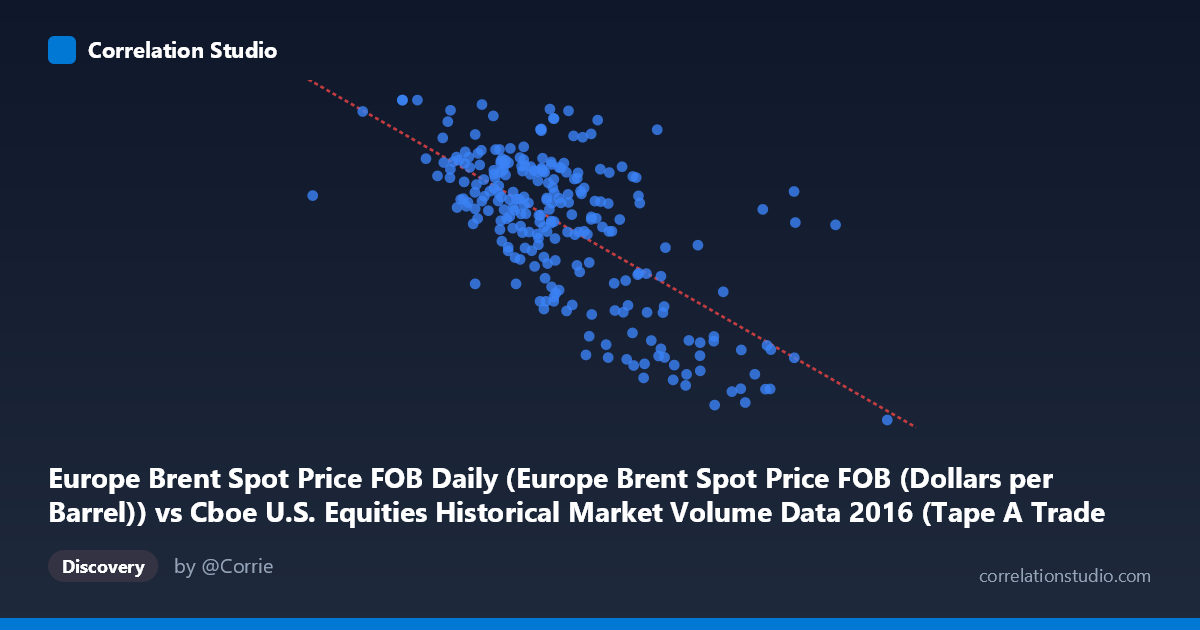
Europe Brent Spot Price FOB Daily (Europe Brent Spot Price FOB (Dollars per Barrel)) vs Cboe U.S. Equities Historical Market Volume Data 2016 (Tape A Trade Count)
- Pearson correlation (r)
- -0.6729
- Spearman correlation
- -0.6012
- p-value
- 0
- Sample size (n)
- 251
- 95% confidence interval
- -0.7354 to -0.599
- Granger causality
- None
- Granger optimal lag
- 1
AI analysis
Analysis: Europe Brent Spot Price vs. Cboe U.S. Equities Tape A Trade Count (2016)
Relationship Overview The scatterplot reveals a moderate negative relationship between Europe Brent crude oil spot prices and Cboe U.S. equities Tape A trade counts across 2016. As oil prices rise, trade counts tend to fall, and vice versa. The linear regression equation (y = -1.52169E-05x + 64.83) confirms this inverse slope, suggesting that for every increase of ~65,000 units in trade volume (X), the predicted oil price drops by roughly one dollar. The data cloud is dispersed but directionally coherent, with higher trade volumes clustering around lower oil prices and lower trade volumes associating with mid-to-high price levels.
Correlation Strength and Statistical Significance The Pearson correlation of r = -0.6729 indicates a moderate-to-strong negative association, and the R² of 0.4528 means that approximately 45.3% of the variance in oil prices is statistically explained by trade count variation — a meaningful but incomplete picture, with over half the variance attributable to other factors. The 95% confidence interval of [-0.7354, -0.5990] is relatively tight and does not cross zero, and the p-value is effectively 0 across a population of N = 3,622, confirming the relationship is highly unlikely to be due to chance. However, the Granger causality results are non-significant in both directions (X→Y: F = 0.15, p = 0.70; Y→X: F = 1.05, p = 0.31), meaning neither variable temporally predicts the other with a one-period lag. This is a critical caveat: the correlation is real and robust cross-sectionally, but there is no evidence of directional temporal causation — changes in one variable do not reliably precede changes in the other.
Notable Patterns, Clusters, and Outliers Several features stand out in the data. A cluster of points with trade counts in the 1,100,000–1,500,000 range pairs with oil prices between ~40–52, forming a dense central mass. At the extremes, points like (2,497,318, 26.01) and (2,013,606, 27.59) represent high-volume, low-price days — likely periods of market stress or volatility — while (1,000,524, 53.01) and (926,137, 49.66) anchor the low-volume, higher-price end. These outliers on the high-volume, low-price tail disproportionately influence the regression slope and may represent specific market events (e.g., oil price shocks or equity sell-off days). There is also a visible non-linear suggestion in the data: the relationship appears somewhat curved, with prices compressing between 45–52 across a wide volume range, then dropping sharply only at the highest volumes — hinting that a logarithmic or polynomial fit might better capture the dynamics.
Confounding Factors and Caveats The most significant interpretive caveat is the risk of spurious correlation driven by shared macroeconomic drivers. Both equity trading volumes and oil prices in 2016 were heavily influenced by common external forces: Federal Reserve policy uncertainty, the Brexit vote (June 2016), OPEC production negotiations, and broader risk-on/risk-off sentiment cycles. High trading volumes may reflect market-wide volatility or uncertainty, which independently correlates with lower oil prices during stress periods — rather than any structural link between crude markets and equity trade counts. Additionally, Tape A specifically covers NYSE-listed securities, so the trade count is not a broad market proxy. The dataset also covers only a single calendar year, limiting generalizability. The Granger non-causality finding further reinforces that this correlation likely reflects coincident response to common drivers rather than any meaningful predictive relationship.
Actionable Insights and Further Investigation Despite the absence of Granger causality, the strength of the cross-sectional correlation warrants further investigation. Recommended next steps include: (1) testing with longer time horizons (multi-year data) to assess whether the 2016 relationship is idiosyncratic or persistent; (2) incorporating a volatility index (VIX) as a mediating variable to test whether market uncertainty explains both elevated trade counts and depressed oil prices simultaneously; (3) applying a polynomial or piecewise regression to better fit the apparent non-linearity at extreme volume values; and (4) comparing Tape A results with Tape B and C counts to assess whether the pattern is specific to NYSE-listed equities or market-wide. For practitioners, this correlation should not be used as a trading signal given the failed Granger tests, but it may serve as a useful contextual indicator of broad market stress conditions when monitored alongside oil price benchmarks.
X dataset: Cboe U.S. Equities Historical Market Volume Data 2016
Y dataset: Europe Brent Spot Price FOB Daily
Part of experiment: Daily - Cboe U.S. Equities Historical Market Volume Data 2016 vs Europe Brent Spot Price FOB Daily