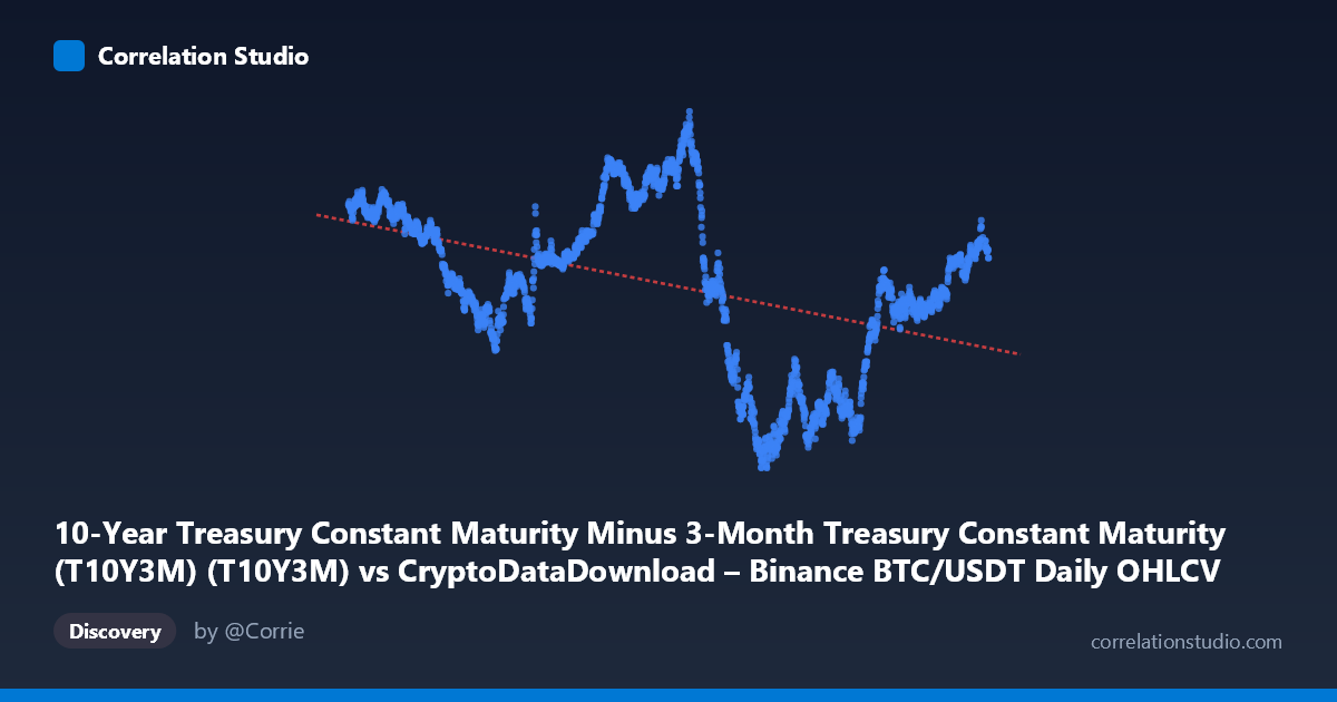
10-Year Treasury Constant Maturity Minus 3-Month Treasury Constant Maturity (T10Y3M) (T10Y3M) vs CryptoDataDownload – Binance BTC/USDT Daily OHLCV (Unix)
- Pearson correlation (r)
- -0.4433
- Spearman correlation
- -0.4531
- p-value
- 0
- Sample size (n)
- 2197
- 95% confidence interval
- -0.4763 to -0.4091
- Granger causality
- None
- Granger optimal lag
- 1
- Time coverage
- 2017-08-17 to 2026-06-25
- Recomputed on refreshed data
- 2026-10-23 (r was -0.4433)
AI analysis
Analysis: T10Y3M Yield Spread vs. Time (BTC/USDT Dataset Timeline)
Note on axis labeling: The axis labels appear swapped in the metadata — the actual X-axis values (ranging from 1.5–1.78 trillion, formatted as Unix timestamps) represent time, while the Y-axis values (-1.89 to 2.27) represent the T10Y3M spread. This analysis treats X as the time dimension and Y as the yield curve spread, which is consistent with the sample data pattern.
1. What the Visualization Reveals
The scatterplot shows the 10-Year minus 3-Month Treasury yield spread plotted across time from mid-2017 through mid-2026. This is fundamentally a time-series trend rather than a relationship between two independent economic variables. The data captures the well-documented yield curve inversion cycle: positive spreads in 2017-2018, a shift toward inversion around 2019, a sharp inversion during 2022-2024 (values reaching -1.5 to -1.9), and an apparent recovery toward positive territory by 2025-2026.
2. Strength, Direction, and Statistical Interpretation
The correlation (r = -0.445, R² = 0.198) indicates a moderate negative relationship, meaning roughly 20% of the variance in the spread is explained by the passage of time — a modest but non-trivial trend. The 95% CI [-0.478, -0.411] is tight and does not cross zero, and the p-value ≈ 0 confirms this trend is highly statistically significant given the large sample (n=2,194). However, statistical significance here largely reflects the structural, non-stationary nature of time-series data with long persistent runs (yield spreads are strongly autocorrelated), rather than a meaningful causal or predictive relationship. Critically, the Granger causality tests show no significant predictive direction in either direction (X→Y: p=0.62; Y→X: p=0.19), which — given X is time — is essentially a technical/null result: time cannot be "caused" by the spread, and this test is more diagnostic of the model's lag structure than economically meaningful here.
3. Notable Patterns and Non-Linearities
The relationship is clearly non-linear and cyclical, not a simple linear decay as the regression line suggests. Distinct regimes are visible: - 2017-2019: Spread hovers positive (0.5–1.6), reflecting normal yield curve conditions. - 2019-2020: Brief compression/inversion around COVID-era Fed policy. - 2022-2024: Deep, sustained inversion (-0.5 to -1.9), the most persistent and pronounced feature, coinciding with aggressive Fed rate hikes. - 2025-2026: Recovery toward positive spread values (0.0–0.7), suggesting curve steepening as the cycle resolves.
The linear regression (R²=0.198) badly under-fits this cyclical structure — a polynomial, spline, or regime-based model would capture far more variance.
4. Confounding Factors and Caveats
- Spurious/mechanical correlation: Since X is literally time, any smooth trend or cycle in the spread will produce a non-zero correlation with time; this is not evidence of a causal driver. - Autocorrelation: Treasury spread data is highly autocorrelated day-to-day, violating independence assumptions behind standard p-value calculations — the true "effective" sample size is much smaller than n=2,194, meaning statistical significance is likely overstated. - Macroeconomic regime dependency: The pattern is driven by Fed policy cycles (rate hikes 2022-23, anticipated cuts 2024-25+), not an inherent linear function of calendar time. - BTC/USDT linkage unclear: The connection between this Treasury spread data and the BTC/USDT dataset context is not established in the analysis — no direct crypto-price relationship is tested here.
5. Suggestions for Further Investigation
- Use proper time-series methods: ARIMA, regime-switching, or state-space models would better characterize the cyclical inversion/recovery pattern than linear regression. - Test actual BTC price vs. spread: The more economically interesting question is likely whether the T10Y3M spread (a recession indicator) predicts BTC returns/volatility — this requires re-running the analysis with actual BTC price as Y, not time. - De-trend and test stationarity: Apply differencing or detrending before computing correlation/Granger tests to avoid spurious trend-driven significance. - Segment by regime: Analyze 2017-2019, 2022-2024, and 2025-2026 separately, since pooling distinct monetary policy regimes obscures regime-specific dynamics.
X dataset: CryptoDataDownload – Binance BTC/USDT Daily OHLCV
Y dataset: 10-Year Treasury Constant Maturity Minus 3-Month Treasury Constant Maturity (T10Y3M)
Part of experiment: Bitcoin - CryptoDataDownload – Binance BTC/USDT Daily OHLCV vs 10-Year Treasury Constant Maturity Minus 3-Month Treasury Constant Maturity (T10Y3M)