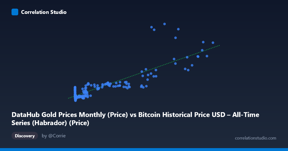
DataHub Gold Prices Monthly (Price) vs Bitcoin Historical Price USD – All-Time Series (Habrador) (Price)
- Pearson correlation (r)
- 0.8497
- Spearman correlation
- 0.6646
- p-value
- 0
- Sample size (n)
- 189
- 95% confidence interval
- 0.8046 to 0.8851
- Granger causality
- None
- Granger optimal lag
- 10
AI analysis
Analysis: Bitcoin Price vs. Gold Price Relationship
1. What the Visualization Reveals
The scatterplot shows a strongly positive but distinctly non-linear relationship between Bitcoin price (X) and gold price (Y). At low Bitcoin values (near-zero to a few thousand dollars, representing Bitcoin's early history 2010–2016), gold prices cluster tightly in the $1,075–$1,900 range with little variance. As Bitcoin climbs into the tens of thousands and beyond (its later bull cycles), gold prices rise more noticeably, reaching $3,000–$5,000+. This pattern is really a time-ordered co-trend rather than a direct causal or mechanistic relationship — both series have risen over the same 2010–2026 window, producing correlation without necessarily reflecting an economic linkage between the two assets on a month-to-month basis.
2. Strength, Direction, and Uncertainty
The Pearson correlation (r = 0.859) is strong, and r² = 0.738 indicates that roughly 74% of the variance in gold prices is statistically "explained" by Bitcoin prices in this linear model. The 95% CI [0.817, 0.893] is tight and the p-value is essentially zero, so the correlation itself is highly reliable — this is not a sampling artifact. However, statistical significance and explanatory power do not imply causal predictive value. The Granger causality tests found no significant directional relationship in either direction (X→Y: p=0.156; Y→X: p=0.773) even at an optimal lag of 10 periods. This is a critical caveat: neither asset's past values help forecast the other's future movements in a time-series sense. The strong contemporaneous r² is likely driven by a shared long-term secular trend (both trending upward over 15+ years) rather than genuine interdependence.
3. Notable Patterns and Outliers
The data is heavily right-skewed in X (mean 20,280 vs. stdev 29,770, max 118,670), so most points cluster at low Bitcoin values with gold in a narrow band (~$1,100–1,900), while a sparser set of high-Bitcoin points pulls the regression line upward. A few notable outliers break the linear pattern: at X≈77,013, Y=5,019.97 (the single highest gold price in the sample, appearing anomalously high relative to neighboring Bitcoin values like X≈85,197 → Y=3,217 or X≈96,467 → Y=3,309). Similarly, X≈65,792 → Y=4,855.54 sits well above the trend of nearby points (e.g., X≈62,440 → Y=2,158). These suggest either genuine gold price spikes (e.g., 2020 pandemic or 2024–2025 safe-haven rallies) decoupled from Bitcoin's concurrent level, or possible data alignment/timestamp issues merging mismatched periods.
4. Confounding Factors and Caveats
The most important confound is time itself: both series are non-stationary trending time series. Macroeconomic drivers — dollar weakness, inflation expectations, quantitative easing, risk-on/risk-off sentiment, and growing institutional adoption of both assets as "alternative stores of value" — plausibly drive both prices upward independently, creating spurious correlation. The linear regression (y = 0.0203x + 1320.52) is a poor structural model given the visible curvature/heteroscedasticity: variance in Y clearly increases with X (fanning out at high Bitcoin values), violating linear regression assumptions. Additionally, comparing a monthly gold series against what appears to be irregularly-spaced Bitcoin data (note the population N=2,319 vs. sampled n=188) raises questions about how the two series were time-aligned/resampled, which could distort the correlation estimate.
5. Actionable Recommendations
Given the non-stationarity, analysts should difference or log-transform both series (e.g., analyze monthly returns rather than price levels) and re-test correlation — this often reveals whether the relationship holds beyond shared trend, or evaporates once trend is removed. The lack of Granger causality strongly suggests these assets should not be used to predict one another's short-term movements; instead, investigate a third common factor (e.g., USD index, real interest rates, or global M2 money supply) that may drive both series. Finally, given the visible outliers and heteroscedasticity, consider a log-log regression or robust/quantile regression to better characterize the relationship at different price regimes, and inspect the data pipeline for potential misalignment between the monthly gold series and the Bitcoin price series.
X dataset: Bitcoin Historical Price USD – All-Time Series (Habrador)
Y dataset: DataHub Gold Prices Monthly
Part of experiment: Bitcoin - Bitcoin Historical Price USD – All-Time Series (Habrador) vs DataHub Gold Prices Monthly