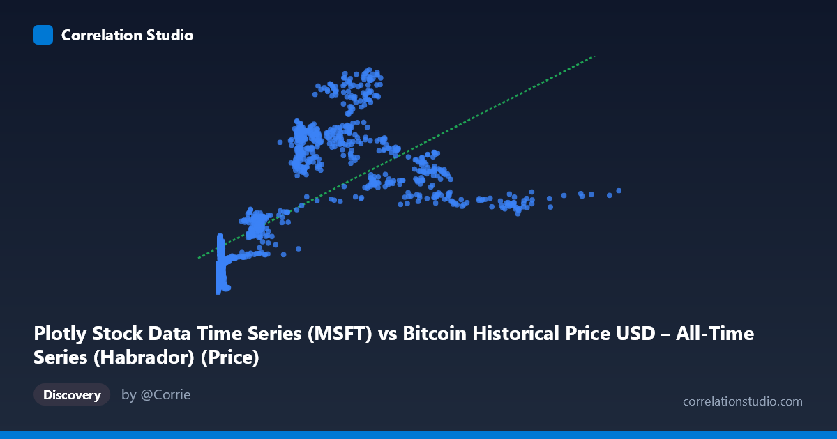
Plotly Stock Data Time Series (MSFT) vs Bitcoin Historical Price USD – All-Time Series (Habrador) (Price)
- Pearson correlation (r)
- 0.6775
- Spearman correlation
- 0.8304
- p-value
- 0
- Sample size (n)
- 1415
- 95% confidence interval
- 0.6483 to 0.7048
- Granger causality
- X → Y
- Granger optimal lag
- 1
- Time coverage
- 2010-07-19 to 2016-03-01
- Recomputed on refreshed data
- 2026-10-24 (r was 0.6775)
AI analysis
Analysis: Bitcoin Price Series vs. MSFT Price Series (Mislabeled Time Series Correlation)
1. What the Visualization Reveals
The scatterplot shows a moderate positive relationship between the two series, with Y values rising from roughly 20-27 at low X values (near zero) to a plateau in the 40-55 range once X exceeds ~200. The data is heavily concentrated at very low X values (many points below X=15), with a long right tail extending to X=1147. This is a classic curved/saturating pattern, not a straight-line relationship — Y increases steeply at first and then flattens, consistent with a logarithmic rather than linear association.
2. Strength, Direction, and Uncertainty
The Pearson correlation (r = 0.6775, r² = 0.459) indicates a moderate-to-strong positive linear relationship, but only about 46% of the variance in Y is explained by X in linear terms — meaning more than half of Y's variability is driven by other factors or by nonlinear structure not captured by a straight line. The 95% CI [0.648, 0.705] is tight, and the p-value is effectively 0, so we can be confident the relationship is real and not due to sampling noise — but statistical significance here reflects the large sample size (n=1,415) more than practical predictive strength. The note that Spearman ρ exceeds Pearson r confirms visual evidence of curvature: a log or polynomial fit would likely explain notably more variance than the 45.9% linear R². On the causality side, the Granger test suggests X leads Y at lag 1 (F=4.73, p=0.03) with no significant reverse effect (p=0.376), implying X's past values have modest predictive value for Y — but this result should be treated cautiously (see caveats below).
3. Notable Patterns and Outliers
- Dense low-X cluster: A large mass of points sits at X < 15 with Y ranging widely (20–28), suggesting high Y variance when X is near zero — this is where the relationship is least deterministic. - Mid-range plateau: From X≈200–700, Y stabilizes in the 34–53 band with substantial scatter (e.g., X=458→Y=51.8 vs. X=572→Y=34.9), indicating no simple 1:1 scaling at higher X. - Sparse tail: Very few points beyond X=700 (max 1147), meaning the upper range is poorly sampled and any trend there is unreliable. - Logarithmic shape: The steep rise then flattening is the hallmark of a log(X) relationship, not linear.
4. Confounding Factors and Caveats
This is critical: the column labels appear swapped or mismatched — X is described as "MSFT" data but sourced from a Bitcoin dataset, while Y is labeled "Bitcoin" but sourced from the Plotly stock dataset. This metadata confusion undermines confident interpretation of what is actually being correlated. Additionally, both series are time series (2010–2016), meaning autocorrelation and shared macro trends (secular growth, market-wide bull runs) can produce spurious correlation even without direct causal linkage — a classic time-series confounding issue. The Granger result, while statistically significant, is a single-lag test on non-stationary financial data, which is prone to false positives unless both series are differenced/detrended first.
5. Actionable Insights
1. Verify data labeling — confirm which variable is actually MSFT vs. Bitcoin before drawing any economic conclusions. 2. Fit a log or polynomial model — given Spearman Pearson and visible curvature, a log(X) transformation will likely raise explained variance substantially above 45.9%. 3. Test stationarity (ADF test) and re-run Granger causality on returns/differenced series rather than raw price levels to rule out spurious trend-driven causality. 4. Segment the analysis by time period or X-range (e.g., low vs. high X) to check if the relationship strength differs across regimes, since the plateau suggests a possible structural break or ceiling effect.
X dataset: Bitcoin Historical Price USD – All-Time Series (Habrador)
Y dataset: Plotly Stock Data Time Series
Part of experiment: Bitcoin - Bitcoin Historical Price USD – All-Time Series (Habrador) vs Plotly Stock Data Time Series