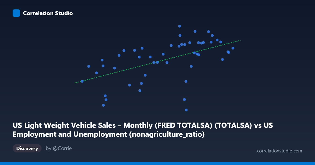
US Light Weight Vehicle Sales – Monthly (FRED TOTALSA) (TOTALSA) vs US Employment and Unemployment (nonagriculture_ratio)
- Pearson correlation (r)
- 0.5326
- Spearman correlation
- 0.5951
- p-value
- 0.000069
- Sample size (n)
- 50
- 95% confidence interval
- 0.2985 to 0.7062
- Granger causality
- None
- Granger optimal lag
- 1
- Time coverage
- 1976-01-01 to 2025-01-01
- Recomputed on refreshed data
- 2026-10-07 (r was 0.5162)
AI analysis
Analysis: US Light Vehicle Sales vs. Non-Agriculture Employment Ratio
Overview of the Relationship
The scatterplot reveals a modest positive relationship between monthly US light-weight vehicle sales (X, measured in thousands of units at a seasonally adjusted annual rate) and the non-agriculture employment ratio (Y). As vehicle sales increase, the non-agriculture employment ratio tends to rise as well, consistent with the intuition that consumer purchasing power and labor market health move together. The linear regression equation (y = 5.21×10⁻⁵x + 8.44) suggests that for every additional 10,000 units in vehicle sales, the employment ratio increases by approximately 0.52 percentage points — a practically meaningful but far from dominant effect.
Correlation Strength and Statistical Significance
The Pearson correlation of r = 0.516 indicates a moderate positive association, but the coefficient of determination r² = 0.267 is the more sobering figure: only 26.6% of the variance in the non-agriculture employment ratio is explained by light vehicle sales. The remaining ~73% reflects forces entirely outside this bivariate model. The 95% confidence interval for r spans [0.278, 0.695], a fairly wide range straddling moderate-to-strong territory, reflecting meaningful uncertainty despite the statistically significant p-value of 0.000125 (well below α = 0.05). With N = 86 population-level observations and n = 50 paired samples spanning 1976–2025, the result is unlikely to be a sampling artifact, but the width of the CI cautions against over-interpretation. Critically, Granger causality analysis reveals no significant predictive direction in either direction (X→Y: F = 0.94, p = 0.34; Y→X: F = 0.66, p = 0.42). This means neither variable reliably predicts the other temporally at a one-period lag — the correlation may reflect co-movement driven by shared underlying forces rather than any direct causal mechanism.
Notable Patterns, Clusters, and Outliers
Several features stand out in the data. There is a visible cluster of points in the upper-right quadrant (sales ~130,000–160,000; employment ratio ~15–18), suggesting a regime of high economic activity where both indicators are simultaneously elevated. Conversely, lower sales figures (85,000–105,000) are associated with more scattered employment ratios ranging broadly from ~10 to ~16, indicating that low vehicle sales periods are more heterogeneous in employment outcomes. At least two noteworthy outliers are apparent: the point near (137,775; 9.79) — high vehicle sales paired with an unusually low employment ratio — and (136,858; 10.89), which similarly disrupts the trend. These anomalies may correspond to structural disruptions (e.g., the 2008–2009 financial crisis or COVID-19 dislocations) where one indicator responded faster than the other.
Confounding Factors and Interpretive Caveats
Several important caveats complicate interpretation. First, both variables are strongly procyclical, meaning they likely co-move with GDP, consumer confidence, and credit conditions rather than directly causing one another — classic confounding by the business cycle. Second, the datasets originate from different measurement frameworks: vehicle sales are monthly SAAR figures while employment data are annual aggregations from BLS, meaning the temporal alignment of paired observations introduces noise. Third, the 49-year time span (1976–2025) encompasses dramatically different economic regimes — stagflation, the Great Moderation, the Great Recession, and pandemic disruptions — and a single linear model may mask substantial structural breaks or regime-dependent relationships. Finally, the non-agriculture employment ratio (as opposed to absolute employment levels) introduces demographic scaling effects that vehicle sales figures do not account for.
Actionable Insights and Further Investigation
Given the moderate correlation and absent Granger causality, this relationship warrants deeper investigation before drawing policy or forecasting conclusions. Recommended next steps include: (1) incorporating GDP or consumer confidence as a covariate to test whether the bivariate correlation is largely mediated by macroeconomic cycles; (2) performing structural break testing (e.g., Chow test) to assess whether the relationship changed after 2008 or 2020; (3) extending the lag structure beyond one period in Granger analysis, as auto-sector employment effects may materialize over 6–12 month horizons rather than a single period; and (4) disaggregating by vehicle type (cars vs. light trucks) or employment sector (manufacturing vs. services) to identify whether the signal concentrates in specific subsectors. The r² of 26.6% leaves substantial room for a richer multivariate model to improve predictive accuracy meaningfully.
X dataset: US Employment and Unemployment
Y dataset: US Light Weight Vehicle Sales – Monthly (FRED TOTALSA)
Part of experiment: Yearly - US Employment and Unemployment vs US Light Weight Vehicle Sales – Monthly (FRED TOTALSA)