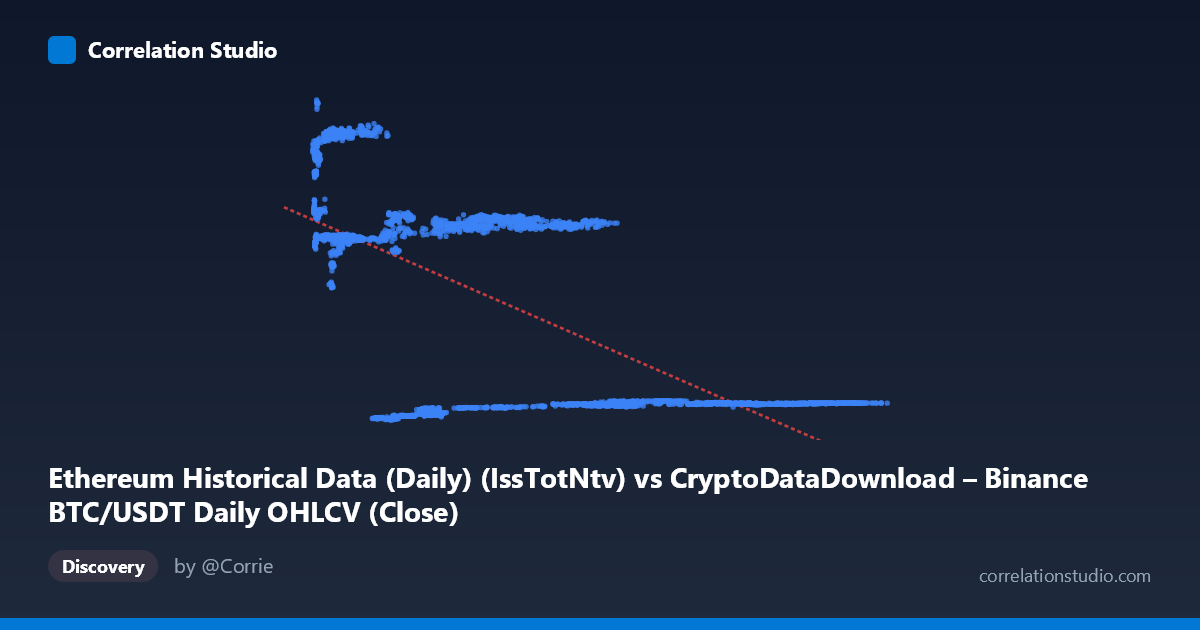
Ethereum Historical Data (Daily) (IssTotNtv) vs CryptoDataDownload – Binance BTC/USDT Daily OHLCV (Close)

Pearson correlation (r): -0.6407
Spearman correlation: -0.4728
p-value: 0
Sample size (n): 3191
95% confidence interval: -0.6607 to -0.6198
Granger causality: Y → X
Granger optimal lag: 10
Time coverage: 2017-08-17 to 2026-05-20

AI analysis

Scatterplot Analysis

1. Overview of the Relationship

The scatterplot depicts a moderately strong negative relationship between the two variables. As X increases, Y tends to decrease, though the data does not form a single tight line — instead, points cluster into several distinct horizontal "bands" (roughly at Y≈2,000-3,000, Y≈13,000-14,500, and Y≈18,000-21,000), each spanning a different range of X values. This banding pattern suggests the underlying relationship may be piecewise, regime-based, or driven by a third factor rather than a smooth continuous decay.

2. Strength, Direction, and Statistical Confidence

The correlation coefficient (r = -0.6407) indicates a moderate-to-strong inverse relationship, with r² = 0.4105 meaning only about 41% of the variance in Y is explained by X — leaving the majority (59%) unexplained by this linear model alone. The 95% confidence interval [-0.6607, -0.6198] is narrow, and the p-value of 0 confirms this correlation is highly statistically significant and not due to chance, largely a function of the very large sample size (n=3,191).

However, statistical significance should not be conflated with strong predictive power — the moderate r² means the linear model leaves substantial variance unexplained. The Granger causality results add an important temporal dimension: Y Granger-causes X (F=1.8667, p=0.0451) at a 10-period lag, while X does NOT Granger-cause Y (F=0.6476, p=0.7737). This suggests that past values of Y (ETH closing price) have modest predictive power for future values of X (BTC's IssTotNtv metric), but not the reverse — implying a unidirectional, lagged predictive relationship rather than simple contemporaneous correlation.

3. Notable Patterns and Clusters

The data clearly separates into at least three horizontal clusters: - Low-Y cluster (~1,500-3,000) spanning a wide X range (roughly 20,000-125,000) — likely representing a later time period with higher/variable BTC network activity but suppressed ETH price. - Mid-Y cluster (~13,000-15,000) concentrated at lower-to-mid X values (roughly 4,000-60,000). - High-Y cluster (~18,000-21,000) concentrated at very low X values (roughly 4,000-13,000).

This stratification strongly suggests time-based regime shifts — likely different market cycles/eras — rather than a continuous functional relationship. The pattern resembles distinct market epochs (e.g., different halving cycles, bull/bear regimes) more than a smooth inverse relationship.

4. Confounding Factors and Caveats

Several caveats are critical here: - Time confound: Both metrics are time-series spanning 2017-2026, a period encompassing multiple BTC/ETH bull and bear markets, halvings, and macro conditions. Apparent correlation likely reflects shared temporal trends rather than direct causal linkage between BTC network issuance and ETH price. - Non-stationarity: Crypto price and network metrics are typically non-stationary (trending, volatile). Granger causality and Pearson correlation assume certain stationarity properties; results may be spurious or unstable without differencing/detrending. - Mismatched variable types: Comparing a BTC network metric (IssTotNtv — total native issuance) to ETH's closing price mixes a supply-side metric with a market price metric, which may not have a coherent causal mechanism. - Clustering effect: The distinct bands suggest a regression run across heterogeneous regimes could produce a misleading "average" linear fit that doesn't represent any single regime well.

5. Actionable Insights and Further Investigation

- Segment by time period/regime: Analyze each visible cluster (band) separately to determine if the negative relationship holds within each era or is purely an artifact of combining distinct market regimes. - Test for stationarity and cointegration: Apply ADF tests and consider differencing both series before re-running correlation/Granger tests to rule out spurious correlation from shared trends. - Investigate the lag-10 Granger result further: Since Y→X causality is only marginally significant (p=0.0451), robustness checks (varying lag lengths, out-of-sample validation) are warranted before treating this as a reliable trading/predictive signal. - Consider a non-linear or piecewise model: Given the banded structure, a regime-switching model or clustering approach (e.g., Gaussian mixture models) may better capture the true structure than a single linear regression.

X dataset: CryptoDataDownload – Binance BTC/USDT Daily OHLCV

Y dataset: Ethereum Historical Data (Daily)

Part of experiment: Bitcoin - CryptoDataDownload – Binance BTC/USDT Daily OHLCV vs Ethereum Historical Data (Daily)