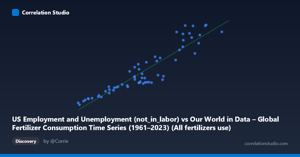
US Employment and Unemployment (not_in_labor) vs Our World in Data – Global Fertilizer Consumption Time Series (1961–2023) (All fertilizers use)
- Pearson correlation (r)
- 0.9247
- Spearman correlation
- 0.925
- p-value
- 0
- Sample size (n)
- 63
- 95% confidence interval
- 0.8782 to 0.9539
- Granger causality
- None
- Granger optimal lag
- 10
- Time coverage
- 1961-01-01 to 2023-01-01
AI analysis
Analysis: US Labor Force Non-Participation vs. Global Fertilizer Consumption (1961–2023)
1. Overall Relationship The scatterplot reveals a strong, positive linear relationship between the number of Americans not in the labor force (X-axis) and global all-fertilizer consumption (Y-axis) across the 1961–2023 period. As the US non-labor-force population grows from roughly 3.2 million to 22.7 million, global fertilizer use rises correspondingly from approximately 48,000 to 100,000 units. The data points cluster reasonably tightly around the regression line (y = 0.00283x + 35,915), suggesting that a simple linear model captures the dominant trend across six decades of joint growth.
2. Correlation Strength and Statistical Framing The Pearson correlation of r = 0.925 is statistically striking, and the R² of 0.855 means that approximately 85.5% of the variance in global fertilizer consumption is statistically "explained" by variation in US non-labor-force participation. The 95% confidence interval for r is narrow at [0.878, 0.954], reinforcing that the correlation estimate is precise and not an artifact of small-sample instability (n = 63, N = 86). The p-value of effectively zero confirms this is not a chance association in a purely statistical sense. However, the Granger causality tests are entirely non-significant in both directions (X→Y: F = 0.728, p = 0.693; Y→X: F = 0.802, p = 0.628) with an optimal lag of 10 periods. This is critical: despite the high correlation, neither variable temporally predicts the other beyond what a naive model would suggest, which is a strong signal that the relationship is driven by a shared underlying trend rather than any causal mechanism linking these two phenomena.
3. Patterns, Clusters, and Notable Features The data broadly separate into two behavioral zones visible in the scatterplot. The lower-left cluster (X < ~8 million, Y < ~62,000) corresponds to earlier decades (1960s–1970s) when both global fertilizer use and US non-participation were lower, while the upper-right region reflects more recent decades of joint expansion. A few notable outliers appear in the upper-right quadrant where fertilizer consumption reaches its highest values (≥95,000 units) at high X values — points such as (22,747,429, 95,716) and (20,610,670, 100,241) — suggesting possible acceleration in fertilizer use in the most recent years that slightly outpaces the linear prediction. There is also modest scatter in the middle range (X ≈ 10–14 million) where Y values spread across roughly 62,000–80,000, hinting at some non-linearity or period-specific variability not captured by the linear model.
4. Confounding Factors and Critical Caveats This correlation is a textbook example of spurious correlation driven by shared secular trends. Both variables are non-stationary time series that grow over time — US non-labor-force participation rises largely due to population growth, aging demographics, and structural labor market shifts, while global fertilizer consumption grows due to expanding agricultural demand, Green Revolution adoption, and rising global population. Time itself is the dominant confound: virtually any two globally or nationally growing quantities measured annually from 1961 to 2023 will exhibit high correlations of this kind. The dataset labels themselves underscore the absurdity of a causal framing — there is no plausible economic, biological, or policy mechanism by which Americans leaving the workforce drives global fertilizer use, or vice versa. The Granger test's failure to find directional predictability further reinforces this. Standard de-trending, first-differencing, or cointegration testing would likely substantially reduce the apparent correlation.
5. Actionable Insights and Further Investigation The primary actionable insight is methodological rather than substantive: analysts working with long-run annual time series must detrend data before interpreting correlation coefficients, as raw levels will almost always produce spuriously high r values. For genuine investigation, first-differencing both series (analyzing year-over-year changes rather than levels) or applying a Hodrick-Prescott filter to isolate cyclical components would provide a more honest test of association. If the research goal involves understanding global fertilizer consumption, more theoretically motivated covariates — global population, real agricultural commodity prices, arable land expansion, or energy prices (given fertilizer's energy intensity) — should be prioritized. Similarly, US labor force trends are better explained by demographic, educational, and disability-related variables. This pairing serves as a useful pedagogical case study in why correlation, confidence intervals, and p-values alone are insufficient without causal theory and time-series stationarity checks.
X dataset: Our World in Data – Global Fertilizer Consumption Time Series (1961–2023)
Y dataset: US Employment and Unemployment
Part of experiment: Yearly - Our World in Data – Global Fertilizer Consumption Time Series (1961–2023) vs US Employment and Unemployment