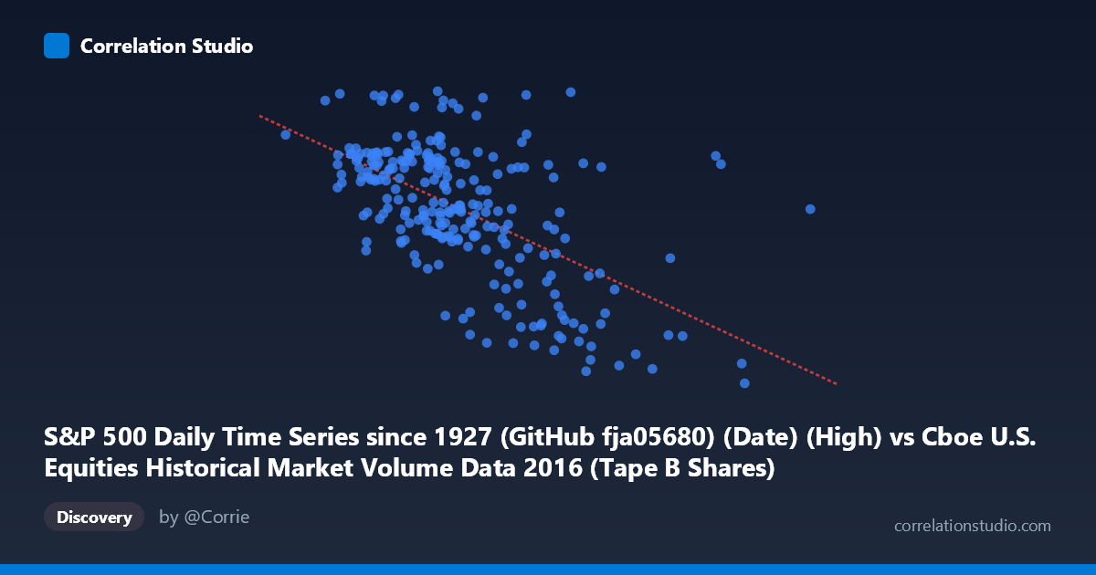
S&P 500 Daily Time Series since 1927 (GitHub fja05680) (Date) (High) vs Cboe U.S. Equities Historical Market Volume Data 2016 (Tape B Shares)
- Pearson correlation (r)
- -0.5819
- Spearman correlation
- -0.5509
- p-value
- 0
- Sample size (n)
- 252
- 95% confidence interval
- -0.6582 to -0.4939
- Granger causality
- None
- Granger optimal lag
- 1
AI analysis
Analysis: S&P 500 Daily High vs. Cboe Tape B Share Volume (2016)
Relationship Overview The scatterplot reveals a moderate negative relationship between the S&P 500 daily high price (X-axis) and Cboe Tape B share volume (Y-axis) across 252 trading days in 2016. As the S&P 500 reached higher price levels, Tape B share volume tended to decline — a pattern that is directionally intuitive but not mechanically tight. The linear regression equation (y = -1.89×10⁻⁶x + 2305.69) captures this downward slope, with the cloud of points showing meaningful scatter around the trend line rather than a clean linear relationship.
Correlation Strength and Statistical Significance The Pearson correlation of r = -0.582 indicates a moderate negative association, and the R² of 0.339 means that approximately 33.9% of the variance in Tape B share volume is explained by the S&P 500 daily high — leaving roughly two-thirds of the variation unexplained by this relationship alone. The 95% confidence interval of [-0.658, -0.494] is relatively narrow and sits entirely in negative territory, providing strong confidence that the true population correlation is meaningfully negative. The p-value of ~0 confirms this is not a chance finding. However, the Granger causality tests are non-significant in both directions (X→Y: F=0.88, p=0.350; Y→X: F=0.77, p=0.381), meaning neither variable temporally predicts the other at a one-period lag. This is a critical caveat: the correlation reflects a contemporaneous co-movement pattern for 2016 rather than any predictive or causal dynamic.
Notable Patterns and Outliers Several features stand out in the data. There is a visible cluster of points concentrated between roughly 75M–115M on the X-axis and 2050–2220 on the Y-axis, suggesting that most trading days in 2016 fell within a relatively bounded range. However, a handful of high-X outliers — particularly around 170M and 233M — correspond to notably low Y values (sub-1950 Tape B volume), pulling the regression slope downward and potentially inflating the correlation. Conversely, some lower X values (e.g., ~78M) show very high Y values near 2270, reinforcing the negative slope. These extremes likely correspond to specific market events (e.g., post-Brexit volatility in late June 2016 or the U.S. election in November), where elevated index highs coincided with unusual volume patterns.
Confounding Factors and Caveats Several important caveats apply. First, Tape B volume represents only a subset of U.S. equity trading (NYSE American-listed securities), not total market volume, so it may respond to sector-specific dynamics rather than broad market conditions. Second, the S&P 500 "High" is a within-day price extreme rather than a closing price, making it a noisier signal. Third, the year 2016 contained several discrete macro shocks (Brexit, U.S. election, Fed rate decisions) that could create spurious correlation by clustering extreme values at particular moments — the relationship may not generalize outside this calendar year. Fourth, the lack of Granger causality suggests this is likely a shared response to common underlying factors (e.g., volatility regimes, risk-off/risk-on sentiment) rather than a direct link between price levels and volume.
Actionable Insights and Further Investigation Given that only ~34% of variance is explained and no temporal predictive relationship exists, practitioners should avoid using S&P 500 daily highs as a standalone predictor of Tape B volume. More productive next steps would include: (1) incorporating the VIX or realized volatility as a mediating variable to test whether the correlation is largely volatility-driven; (2) extending the analysis beyond 2016 to test whether this negative relationship is stable across different market regimes; (3) examining whether total Cboe volume or Tape A/C volumes show a similar pattern; and (4) running a multivariate regression adding day-of-week effects, macroeconomic announcement days, and volume from prior sessions to better isolate what drives Tape B share volume. The correlation is real and statistically robust for 2016, but its practical utility depends on understanding why it exists — likely through shared sensitivity to market stress and liquidity conditions.
X dataset: Cboe U.S. Equities Historical Market Volume Data 2016
Y dataset: S&P 500 Daily Time Series since 1927 (GitHub fja05680) (Date)
Part of experiment: Daily - Cboe U.S. Equities Historical Market Volume Data 2016 vs S&P 500 Daily Time Series since 1927 (GitHub fja05680) (Date)