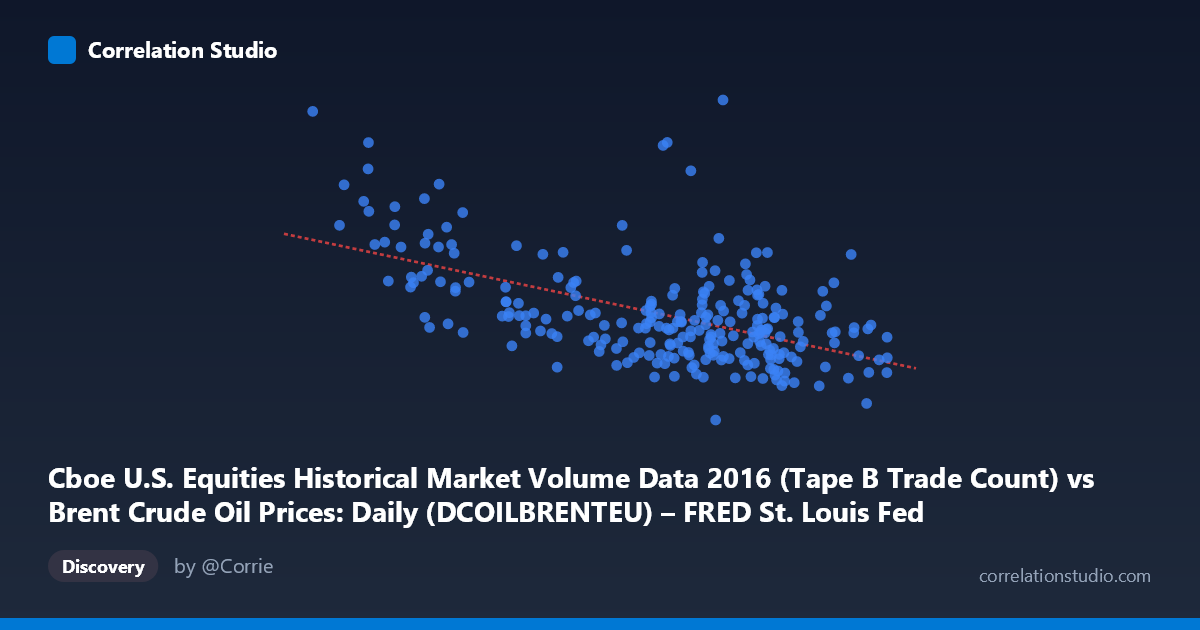
Cboe U.S. Equities Historical Market Volume Data 2016 (Tape B Trade Count) vs Brent Crude Oil Prices: Daily (DCOILBRENTEU) – FRED St. Louis Fed (DCOILBRENTEU)
- Pearson correlation (r)
- -0.5472
- Spearman correlation
- -0.4797
- p-value
- 0
- Sample size (n)
- 251
- 95% confidence interval
- -0.6285 to -0.4542
- Granger causality
- None
- Granger optimal lag
- 10
AI analysis
Analysis: Brent Crude Oil Price vs. Cboe Tape B Trade Count (2016)
Relationship Overview The scatterplot reveals a moderate negative relationship between Brent Crude Oil prices (X-axis, USD/barrel) and Cboe U.S. Equities Tape B trade counts (Y-axis). The linear regression equation y = -7,765.19x + 658,900 indicates that for every $1 increase in Brent crude price, trade count decreases by approximately 7,765 units. Visually, the data points show a downward-sloping trend, with higher crude prices (around $48–55/barrel) clustering around lower trade counts (roughly 200,000–350,000), while lower crude prices (around $26–34/barrel) are associated with substantially higher trade counts (400,000–700,000). This inverse pattern suggests that periods of depressed oil prices in 2016 coincided with elevated equity trading activity, possibly reflecting heightened market uncertainty and volatility.
Correlation Strength and Statistical Significance The Pearson correlation of r = -0.547 indicates a moderate negative association, but the variance explained (r² = 0.2995) clarifies that only ~30% of the variance in trade counts is attributable to crude oil price movements, meaning roughly 70% of trade count variability stems from other factors entirely. The 95% confidence interval of [-0.629, -0.454] is meaningfully narrow and entirely negative, providing strong statistical confidence that the inverse relationship is real and not a sampling artifact. The p-value of effectively 0 (against N = 3,622) confirms this is highly unlikely to be a chance finding. However, the Granger causality results tell a critically different story: neither direction (X→Y nor Y→X) achieves significance (F = 0.715, p = 0.710 and F = 0.686, p = 0.737 respectively at the optimal 10-period lag), meaning that neither variable temporally predicts the other. This firmly distinguishes statistical correlation from any predictive or causal mechanism — the two variables move together, but neither leads the other.
Notable Patterns and Outliers Several prominent outliers are visible in the lower-price range. Points near X = 26–28 (Brent around $26–$28/barrel) show extremely elevated trade counts reaching 558,000–714,000, substantially above the regression line and consistent with the historic oil price crash of early 2016. These leverage points likely exert disproportionate influence on the regression slope and the overall r value. Conversely, a cluster of points between X = 44–52 shows considerable vertical scatter (trade counts ranging from ~190,000 to ~433,000 at similar price levels), indicating high unexplained variability in the mid-to-high price range. The relationship also appears potentially non-linear — the dramatic trade count spikes at very low prices suggest a possible exponential or threshold effect rather than a purely linear relationship, and the residuals in the mid-price range appear relatively flat.
Confounding Factors and Caveats Several important caveats limit causal interpretation. First, both variables are time-series data from 2016, meaning shared temporal trends, seasonality, and macro events (e.g., OPEC decisions, Fed rate policy, Brexit in June 2016) could be driving both variables simultaneously without any direct linkage. Second, the Tape B trade count reflects a specific exchange segment, which may be influenced by platform-specific factors entirely unrelated to commodity markets. Third, early 2016 represented an extraordinary period of global market stress — the oil price nadir created unusual volatility across asset classes, which could inflate the correlation artificially beyond what would be observed in calmer periods. The large population size (N = 3,622 vs. sample n = 251) also warrants careful consideration of whether the sample captures the full distributional range representatively.
Actionable Insights and Further Investigation Given the lack of Granger causality, practitioners should resist using crude oil prices as a timing signal for equity trading volume predictions. However, the moderate correlation and the striking outlier behavior at extreme oil price levels warrant deeper investigation. Recommended next steps include: (1) testing a non-linear (log or polynomial) regression model to better capture the apparent threshold effect at low oil prices; (2) introducing macro control variables such as the VIX volatility index, USD index, or S&P 500 returns to isolate whether the correlation persists after controlling for broader market stress; (3) segmenting the analysis by market regime (e.g., pre/post OPEC announcement dates) to test whether the correlation is regime-dependent; and (4) examining whether other Tape segments (A and C) show similar patterns, which would help distinguish whether this is an equity market phenomenon broadly or specific to Tape B securities. The 2016 time window is narrow and unusual — replicating this analysis across multiple years would substantially strengthen or weaken confidence in the observed relationship.
X dataset: Brent Crude Oil Prices: Daily (DCOILBRENTEU) – FRED St. Louis Fed
Y dataset: Cboe U.S. Equities Historical Market Volume Data 2016
Part of experiment: Daily - Brent Crude Oil Prices: Daily (DCOILBRENTEU) – FRED St. Louis Fed vs Cboe U.S. Equities Historical Market Volume Data 2016