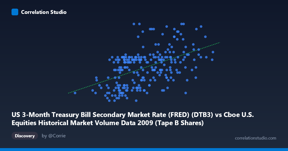
US 3-Month Treasury Bill Secondary Market Rate (FRED) (DTB3) vs Cboe U.S. Equities Historical Market Volume Data 2009 (Tape B Shares)
- Pearson correlation (r)
- 0.4942
- Spearman correlation
- 0.5039
- p-value
- 0
- Sample size (n)
- 250
- 95% confidence interval
- 0.3943 to 0.5825
- Granger causality
- None
- Granger optimal lag
- 1
AI analysis
Analysis: US 3-Month T-Bill Rate vs. Cboe Tape B Share Volume (2009)
Relationship Overview The scatterplot reveals a moderate positive relationship between the US 3-Month Treasury Bill Secondary Market Rate and Cboe Tape B equity share volume during 2009. As T-bill rates increase, Tape B share volume tends to rise, consistent with the positive regression slope (y = 8.13×10⁻¹⁰x + 0.031). This relationship is financially intuitive in the context of 2009's post-crisis environment, where both variables were simultaneously responding to rapidly shifting macroeconomic conditions — particularly the Federal Reserve's aggressive rate interventions and the volatile equity market recovery following the March 2009 trough.
Correlation Strength and Statistical Significance The Pearson correlation of r = 0.494 indicates a moderate positive association, but the explanatory power is limited: r² = 0.244 means only ~24.4% of variance in Tape B volume is explained by T-bill rates, leaving roughly 75.6% attributable to other factors. The 95% confidence interval of [0.394, 0.583] is reasonably tight given n=250, and the p-value of effectively zero confirms this correlation is highly unlikely to be a chance artifact. However, the Granger causality tests reveal no significant temporal predictive direction in either direction (X→Y: F=0.488, p=0.486; Y→X: F=0.384, p=0.536). This critical finding means that neither variable reliably predicts the other with a one-period lag — the observed correlation likely reflects contemporaneous co-movement driven by shared external drivers, not a causal mechanism between the two series.
Notable Patterns and Outliers Several features stand out in the sample points. There is notable vertical dispersion at mid-range X values (~100M–175M), where Y spans nearly the full range (0.03–0.30), suggesting the relationship weakens considerably in the middle of the T-bill rate distribution. A cluster of low-volume, low-rate observations appears at the lower-left (e.g., 33.8M/0.05, 66.8M/0.05, 82.6M/0.04), consistent with the post-Lehman near-zero rate environment early in 2009. Conversely, higher-volume observations (e.g., 205M/0.32, 243M/0.27, 198M/0.29) cluster at elevated X values, pulling the regression slope upward. The point at (254.5M, 0.18) appears as a potential high-leverage outlier on the X-axis that may disproportionately influence the regression fit.
Confounding Factors and Caveats The most significant caveat is temporal confounding: both series are time-indexed daily observations across 2009, meaning the correlation may largely capture the shared temporal trend of a recovering economy rather than any direct functional relationship. The March 2009 market bottom, quantitative easing announcements, and TARP unwinding all created synchronized movements across virtually all financial variables simultaneously. Additionally, Tape B volume (covering NYSE American and regional exchanges) may be influenced by ETF rebalancing, algorithmic trading patterns, and exchange market share dynamics that have no mechanistic connection to T-bill rates. The low Granger F-statistics further reinforce that this is likely a spurious or indirect correlation mediated through macroeconomic recovery dynamics.
Actionable Insights and Further Investigation Given the absence of Granger causality and moderate r², practitioners should avoid using T-bill rates as a direct predictor of Tape B volume in short-term trading models. Further investigation should include: (1) detrending both series to remove the shared 2009 recovery trend and re-testing correlation on residuals; (2) introducing VIX or S&P 500 returns as control variables to test whether the correlation disappears once market sentiment is accounted for; (3) extending the analysis across multiple years to determine whether this relationship is specific to the crisis-recovery period or persists structurally; and (4) testing longer Granger lags (beyond 1 period) to see if delayed predictive relationships emerge at weekly or monthly frequencies.
X dataset: Cboe U.S. Equities Historical Market Volume Data 2009
Y dataset: US 3-Month Treasury Bill Secondary Market Rate (FRED)
Part of experiment: Daily - Cboe U.S. Equities Historical Market Volume Data 2009 vs US 3-Month Treasury Bill Secondary Market Rate (FRED)