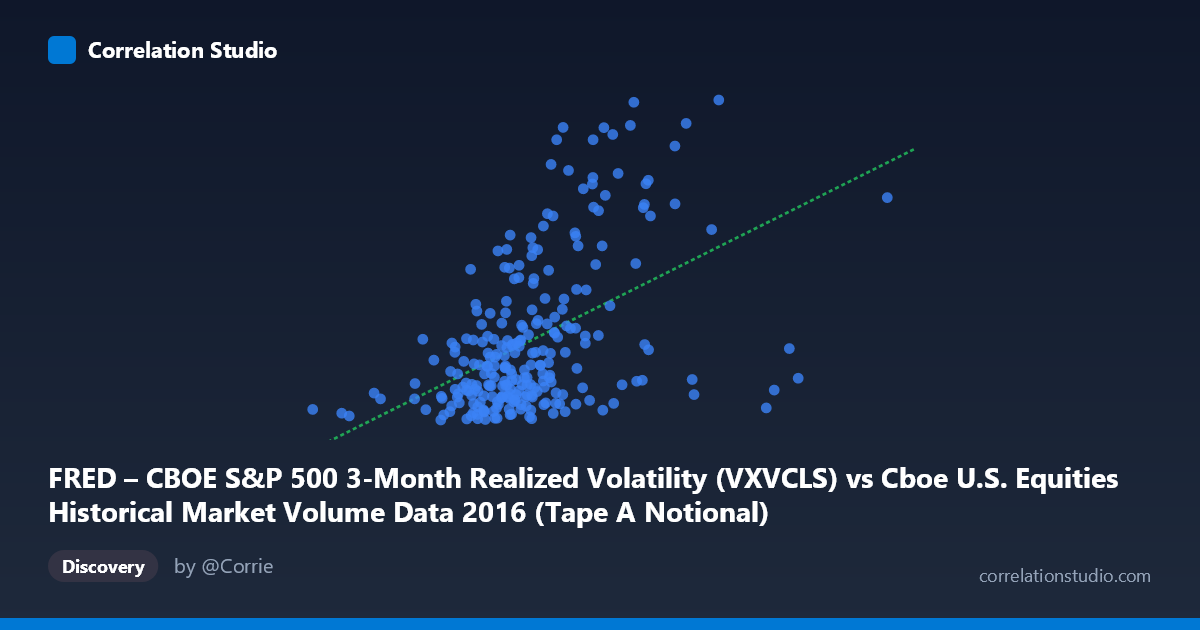
FRED – CBOE S&P 500 3-Month Realized Volatility (VXVCLS) vs Cboe U.S. Equities Historical Market Volume Data 2016 (Tape A Notional)
- Pearson correlation (r)
- 0.4761
- Spearman correlation
- 0.4708
- p-value
- 0
- Sample size (n)
- 252
- 95% confidence interval
- 0.3745 to 0.5663
- Granger causality
- None
- Granger optimal lag
- 1
AI analysis
Scatterplot Analysis: CBOE S&P 500 3-Month Realized Volatility vs. Tape A Notional Volume (2016)
Relationship Overview
The scatterplot reveals a moderate positive relationship between CBOE S&P 500 3-Month Realized Volatility (VXVCLS) and Tape A Notional trading volume across 2016. As equity market volume (X) increases, realized volatility (Y) tends to rise as well. The linear regression equation (y = 8.16×10⁻¹⁰x + 10.93) confirms this upward slope, and the scatter of points makes the trend discernible but far from tight. There is clearly substantial dispersion around the regression line, suggesting meaningful variation in volatility that volume alone does not capture. The relationship is broadly consistent with market microstructure intuition: elevated trading activity often accompanies — and reflects — periods of heightened uncertainty and price instability.
Correlation Strength, Significance, and Temporal Direction
The Pearson correlation of r = 0.4761 indicates a moderate positive association. However, the coefficient of determination r² = 0.2266 tells the more sobering story: only about 22.7% of the variance in realized volatility is explained by notional volume, leaving roughly 77% attributable to other factors. The 95% confidence interval [0.3745, 0.5663] is reasonably tight and excludes zero entirely, and the p-value of 1.11×10⁻¹⁵ confirms this correlation is highly statistically significant — extremely unlikely to be a chance finding given n = 252 paired observations drawn from N = 3,622. Despite this statistical robustness, the Granger causality results are notably null in both directions: X→Y (F = 0.0007, p = 0.9794) and Y→X (F = 0.941, p = 0.333). This means that while volume and volatility move together contemporaneously, neither variable reliably predicts the other in subsequent periods at a one-period lag. Correlation here appears to reflect co-movement driven by shared underlying forces rather than any directional, temporal predictive relationship.
Patterns, Clusters, and Outliers
The sample points reveal several structurally interesting features. The bulk of observations cluster between roughly 7.5–10.5 billion in volume and 15–20 in volatility, forming a dense core consistent with "normal" market conditions during 2016's relatively calm mid-year period. However, there is a visually distinct upper-right cluster of outliers — points such as (10,752,811,050; 26.71), (9,467,293,564; 25.25), and (10,473,202,410; 24.47) — where both volume and volatility spike simultaneously. These likely correspond to identifiable market stress events in 2016 (e.g., Brexit in late June, the U.S. presidential election in November), when fear-driven volume surged alongside volatility. Conversely, there are points with moderately high volume but low volatility (e.g., 11,550,248,214; 16.63), suggesting volume can be elevated without commensurate volatility — perhaps reflecting routine institutional rebalancing. The presence of these regime-like clusters hints that a single linear model may be oversimplifying a more conditional or piecewise relationship.
Confounding Factors and Interpretive Caveats
Several important caveats temper interpretation. First, note the axis assignment: the dataset labels are cross-applied — the X-axis draws from the CBOE volatility dataset and the Y-axis from the volume dataset — which may reflect an intentional analytical choice but warrants scrutiny to ensure variables are correctly mapped to their conceptual roles. Second, reverse causality is plausible: high volatility may trigger algorithmic and hedging activity that itself inflates volume, meaning the causal arrow could run in either direction or be bidirectional — yet Granger tests at lag 1 rule out clean temporal precedence. Third, macroeconomic regime effects (e.g., central bank announcements, geopolitical shocks) likely drive both variables simultaneously, making the observed correlation largely a spurious co-movement artifact of shared external drivers rather than an intrinsic volume-volatility mechanism. Finally, the daily sampling frequency and 2016 calendar year scope limit generalizability; this relationship may behave differently across longer horizons or distinct market regimes.
Actionable Insights and Further Investigation
Despite the null Granger result, the contemporaneous correlation is practically meaningful and suggests several avenues for deeper work. Event-stratified analysis — separating Brexit, election, and Fed announcement days from calm periods — would likely reveal whether the correlation is driven disproportionately by a small number of stress episodes, which would have major implications for risk models. Practitioners in volatility trading or market-making should note that while volume cannot predict next-period volatility, the two rising together in real-time can serve as a concurrent regime signal. Non-linear modeling (e.g., quantile regression or regime-switching models) could better capture the apparent threshold behavior where high-volume days bifurcate into high- and low-volatility outcomes. Finally, incorporating additional explanatory variables — such as the VIX term structure, order flow imbalance, or macroeconomic surprise indices — would likely substantially close the 77% unexplained variance gap and yield a more actionable predictive framework.
X dataset: Cboe U.S. Equities Historical Market Volume Data 2016
Y dataset: FRED – CBOE S&P 500 3-Month Realized Volatility
Part of experiment: Daily - Cboe U.S. Equities Historical Market Volume Data 2016 vs FRED – CBOE S&P 500 3-Month Realized Volatility