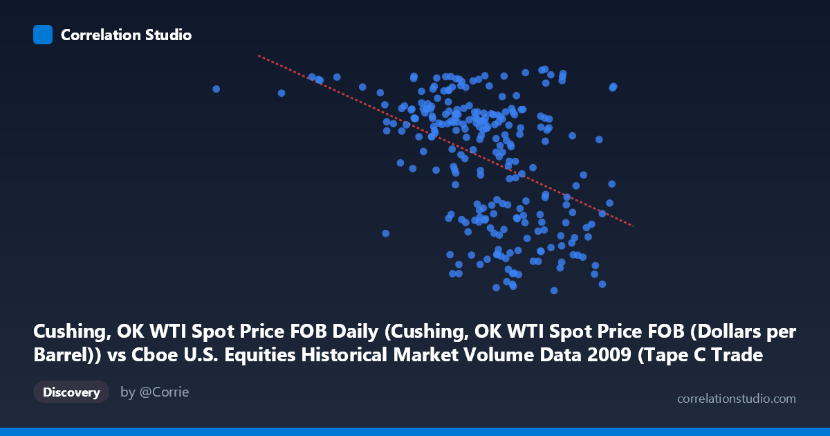
Cushing, OK WTI Spot Price FOB Daily (Cushing, OK WTI Spot Price FOB (Dollars per Barrel)) vs Cboe U.S. Equities Historical Market Volume Data 2009 (Tape C Trade Count)
- Pearson correlation (r)
- -0.4325
- Spearman correlation
- -0.43
- p-value
- 0
- Sample size (n)
- 252
- 95% confidence interval
- -0.5279 to -0.3264
- Granger causality
- None
- Granger optimal lag
- 1
AI analysis
Analysis: WTI Crude Oil Price vs. Cboe Tape C Trade Count (2009)
Relationship Overview
The scatterplot reveals a moderate negative relationship between WTI crude oil spot prices (X-axis, in dollars per barrel) and Cboe Tape C trade counts (Y-axis). As oil prices increase, trade counts in the Tape C segment tend to decrease. The linear regression equation (y = -5.79×10⁻⁵x + 98.77) captures this downward slope, though the scatter around the regression line is substantial, indicating that oil price alone is a weak-to-moderate predictor of equity trading volume in this segment. The data spans the full calendar year 2009 — a period of significant macroeconomic turbulence following the 2008 financial crisis, which adds important context to any patterns observed.
Correlation Strength, Direction, and Statistical Significance
The Pearson correlation of r = -0.4325 indicates a moderate negative association. However, the coefficient of determination R² = 0.1871 is the more practically revealing statistic: it means that only ~18.7% of the variance in Tape C trade counts is explained by variation in WTI prices, leaving roughly 81% of variance attributable to other factors. The 95% confidence interval for r of [-0.5279, -0.3264] is reasonably tight and does not include zero, and the p-value of 6.54×10⁻¹³ confirms the correlation is highly statistically significant given the sample size of 252 paired observations. That said, statistical significance here is partly a function of sample size (N = 3,232 population), and the effect size remains modest. Critically, the Granger causality tests reveal no significant predictive directionality in either direction — neither X→Y (F = 1.36, p = 0.24) nor Y→X (F = 1.82, p = 0.18) achieves significance at conventional thresholds — meaning WTI prices do not temporally predict Tape C trade counts, nor vice versa, at a one-period lag. This strongly cautions against interpreting the correlation as reflecting a causal or predictive mechanism.
Notable Patterns, Clusters, and Outliers
Several structural features stand out in the scatterplot. There appears to be a wide vertical spread at lower oil price values (roughly $35–$55/barrel), suggesting high variability in trade counts when oil is cheap. At higher price ranges (~$70–$85/barrel), trade counts show less dispersion and tend to concentrate in lower ranges, which is consistent with the negative slope but also hints at a possible non-linear or heteroscedastic relationship rather than a clean linear one. A notable outlier cluster appears in the lower-left region — very low oil prices paired with mid-to-high trade counts — which may correspond to the early 2009 period when oil prices had collapsed post-crisis and equity trading volumes were elevated due to market volatility and panic activity. The point at (185,886.83, 76.83) appears to be a pronounced outlier on the X-axis and may represent an anomalous or misscaled observation worth investigating. There also appears to be a bifurcation in the data at mid-price ranges, with two bands of trade counts visible, possibly reflecting a structural shift in market behavior across the year.
Confounding Factors and Interpretive Caveats
The 2009 timeframe is a critical caveat. This was a year of extreme macroeconomic stress — the economy was in recession through mid-year, equity markets bottomed in March before rebounding sharply, and oil prices were recovering from their 2008 collapse. These shared macroeconomic drivers (risk appetite, investor sentiment, economic recovery expectations) could easily produce a spurious negative correlation between oil prices and trade counts without any direct mechanistic link. Additionally, Tape C specifically covers NYSE Arca-listed securities, which skews toward ETFs and certain equities that may respond differently to oil price movements than the broader market. The absence of Granger causality at a one-period lag also raises the possibility that any relationship operates at longer lags or through indirect channels not captured here, or that both variables are independently driven by a common latent factor such as macroeconomic uncertainty or market volatility (e.g., VIX).
Actionable Insights and Further Investigation
Given the modest explanatory power and absent Granger causality, practitioners should not use WTI prices as a standalone predictor of Tape C trading activity. However, the correlation is strong enough to warrant deeper investigation. Recommended next steps include: (1) Introducing a volatility proxy (e.g., VIX) as a control variable to test whether the oil–trade count relationship is mediated by market uncertainty; (2) Testing multiple Granger lags (beyond the single period tested here) to check for delayed predictive relationships; (3) Segmenting the analysis by sub-period (e.g., Q1 crisis phase vs. Q3–Q4 recovery) to determine whether the negative correlation is regime-dependent; (4) Examining non-linear models (e.g., spline regression or quantile regression) given the apparent heteroscedasticity; and (5) Cross-validating against other Tape segments (A and B) to determine whether the pattern is specific to Tape C or reflects a broader equity market dynamic. Together, these steps would help distinguish genuine economic linkage from shared-crisis confounding.
X dataset: Cboe U.S. Equities Historical Market Volume Data 2009
Y dataset: Cushing, OK WTI Spot Price FOB Daily
Part of experiment: Daily - Cboe U.S. Equities Historical Market Volume Data 2009 vs Cushing, OK WTI Spot Price FOB Daily