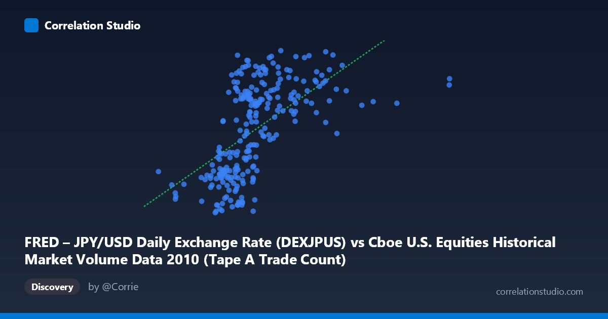
FRED – JPY/USD Daily Exchange Rate (DEXJPUS) vs Cboe U.S. Equities Historical Market Volume Data 2010 (Tape A Trade Count)
- Pearson correlation (r)
- 0.59
- Spearman correlation
- 0.6741
- p-value
- 0
- Sample size (n)
- 249
- 95% confidence interval
- 0.5025 to 0.6655
- Granger causality
- None
- Granger optimal lag
- 1
AI analysis
Scatterplot Analysis: JPY/USD Exchange Rate vs. Cboe Tape A Trade Count (2010)
Relationship Overview
The scatterplot reveals a moderate positive relationship between the JPY/USD daily exchange rate and Cboe U.S. Equities Tape A trade counts during 2010. As the yen-per-dollar rate increases (meaning the dollar strengthens relative to the yen), Tape A trade counts tend to rise as well. The linear regression equation (y = 6.207×10⁻⁶x + 79.54) reflects a shallow but consistent upward slope across the observed range, with the bulk of observations clustering between approximately 900,000–1,600,000 on the X-axis and 83–93 on the Y-axis. This positive co-movement is visually apparent, though substantial scatter around the regression line is evident throughout.
Correlation Strength and Statistical Interpretation
The Pearson correlation of r = 0.59 indicates a moderate positive association, but the R² of 0.3481 is the more sobering metric: only 34.8% of the variance in Tape A trade counts is explained by the JPY/USD rate. The remaining ~65% is driven by factors entirely unrelated to this exchange rate. The 95% confidence interval of [0.503, 0.666] is reasonably tight given the sample size (n = 249, N = 3,302), and the p-value of effectively zero confirms this correlation is not a chance artifact. However, statistical significance with large N should not be conflated with practical importance. Critically, Granger causality testing finds no significant predictive directionality in either direction — neither X→Y (F = 1.32, p = 0.25) nor Y→X (F = 0.68, p = 0.41) — meaning that past values of one variable do not meaningfully forecast the other at a one-period lag. This decisively limits any causal or predictive narrative between these two series.
Patterns, Clusters, and Outliers
Several notable structural features are visible in the data. A dense central cluster sits in the 1,000,000–1,500,000 exchange rate range with trade counts between roughly 83 and 93, suggesting this was the modal operating environment for 2010 markets. There are visible outliers on the upper-right of the X-axis — observations near 2,000,000–3,200,000 — which represent either extreme volume days or data anomalies, and some of these do not conform neatly to the regression line, potentially inflating the correlation. On the lower end, a sparse tail below 600,000 (including one observation near 508,819) exists in relative isolation. The distribution also appears to show heteroscedasticity: scatter in the Y-direction widens at higher X values, suggesting the linear model fits less reliably at the extremes. There is also a hint of a non-linear or bimodal structure — points at middle X values span the full Y range, complicating a strictly linear interpretation.
Confounding Factors and Caveats
This correlation almost certainly reflects shared temporal structure rather than a direct economic mechanism. Both series are daily time series from calendar year 2010, and any common macro-financial trends — risk sentiment cycles, the European sovereign debt crisis, post-financial crisis market normalization — could simultaneously drive both equity trading volumes and the yen/dollar rate without one causing the other. The JPY/USD rate is plotted on the X-axis and labeled as coming from the Cboe volume dataset, while Tape A trade count is sourced from the FRED dataset — this axis-label cross-labeling warrants careful verification of the data merge. Additionally, the mismatch between population (N = 3,302) and sample (n = 249) suggests aggregation or sampling choices that could introduce selection bias. The lack of Granger causality at lag-1 also hints that any shared movement is contemporaneous and driven by a third common factor, not by sequential influence.
Actionable Insights and Further Investigation
Given the absence of Granger causality, practitioners should avoid using JPY/USD rates as a leading indicator for Tape A trade volumes (or vice versa) in any trading or operational model. The ~35% explained variance does suggest a meaningful common factor worth identifying — likely broad risk-on/risk-off sentiment or dollar strength indices that simultaneously affect FX markets and equity participation. Further investigation should include: (1) testing additional Granger lags beyond 1 period; (2) introducing control variables such as VIX, S&P 500 returns, or Fed policy event dummies to decompose the shared variance; (3) applying a rolling-window correlation analysis to determine whether this relationship was stable across 2010 or concentrated in specific sub-periods; and (4) verifying the data axis assignments to ensure the cross-dataset merge is correctly aligned temporally before drawing any further conclusions.
X dataset: Cboe U.S. Equities Historical Market Volume Data 2010
Y dataset: FRED – JPY/USD Daily Exchange Rate
Part of experiment: Daily - Cboe U.S. Equities Historical Market Volume Data 2010 vs FRED – JPY/USD Daily Exchange Rate