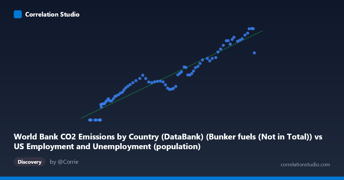
World Bank CO2 Emissions by Country (DataBank) (Bunker fuels (Not in Total)) vs US Employment and Unemployment (population)
- Pearson correlation (r)
- 0.9596
- Spearman correlation
- 0.971
- p-value
- 0
- Sample size (n)
- 80
- 95% confidence interval
- 0.9376 to 0.974
- Granger causality
- None
- Granger optimal lag
- 10
AI analysis
Scatterplot Analysis: Bunker Fuel CO₂ Emissions vs. US Employment Population
1. Overall Relationship The scatterplot reveals a strong, predominantly positive linear relationship between international bunker fuel CO₂ emissions and the US employment population over the period 1941–2020. As bunker fuel emissions increase across the X-axis range (~93,000 to ~260,000 units), US employment population rises correspondingly from near zero to approximately 1,590 units. The fitted linear regression (y = 0.00827x − 669.17) captures this trend well, though a notable cluster of zero-valued Y observations at the lower end of X suggests either a threshold effect or data censoring in the early historical period, introducing a mild non-linearity at the left tail.
2. Correlation Strength, Direction, and Causality The Pearson correlation of r = 0.9596 is exceptionally strong and positive, with R² = 0.921, meaning approximately 92.1% of the variance in US employment population is statistically explained by bunker fuel emissions within this sample. The 95% confidence interval [0.9376, 0.9740] is narrow and does not approach zero, and the p-value of effectively 0 confirms this is not a chance association at any conventional significance threshold. However, the Granger causality analysis tells a critical story: neither direction (X→Y: F=1.74, p=0.099; Y→X: F=1.51, p=0.166) achieves statistical significance at the 0.05 level, even at the optimal lag of 10 periods. This means that despite the powerful correlation, neither variable demonstrably predicts the other temporally — past values of bunker emissions do not forecast future US employment levels, and vice versa. The relationship is associative, not directionally predictive.
3. Notable Patterns, Clusters, and Outliers Several observations stand out. First, there is a distinct cluster of zero Y-values (at least 7–8 points) concentrated in the lower X range (~93,000–104,000), likely corresponding to the early 1940s when employment data collection or reporting may have used different baselines. Second, the data broadly separates into two behavioral regimes: a sparse, lower-emission/lower-employment zone and a dense, higher-emission/higher-employment cloud that follows the regression line closely. The point at (260,329; 1,168.54) appears as a moderate outlier, sitting noticeably below the regression line given its high X value — this may represent a post-2015 period where emissions plateaued or declined while employment continued growing. Points near (257,791; 1,591.53) and (259,175; 1,589.59) align well with expectations at the upper extreme.
4. Confounding Factors and Interpretive Caveats The most important caveat here is spurious correlation driven by shared temporal trends. Both bunker fuel emissions and US employment population have grown substantially over the 80-year study period, largely as functions of global economic expansion, population growth, and industrialization — classic cases of variables that co-move not because they cause each other, but because both are driven by the same underlying macro forces (GDP growth, globalization, post-WWII economic expansion). The zero-floor cluster may also reflect data artifact rather than true behavior, inflating apparent linearity. Additionally, the dataset pairing itself is conceptually unusual — bunker fuels represent international shipping/aviation emissions categorized as "not in national totals," making a direct mechanistic link to US domestic employment particularly indirect. The mismatch between dataset labels (X labeled as coming from "US Employment" dataset, Y from "CO₂ DataBank") suggests possible column misattribution worth verifying.
5. Actionable Insights and Further Investigation Given the absence of Granger causality, analysts should resist any policy or forecasting inference that bunker fuel trends can predict US labor market conditions or vice versa. Recommended next steps include: (a) introducing GDP, global trade volume, or population as explicit control variables to test whether the correlation survives partial regression; (b) applying cointegration analysis (e.g., Engle-Granger or Johansen tests) to determine if a long-run equilibrium relationship exists beyond shared trending; (c) investigating the outlier at X≈260,000 to determine if it represents a structural break in the post-2015 era of decarbonization efforts; and (d) verifying the dataset column assignments, as the cross-labeling of source datasets raises data provenance concerns that could affect all downstream conclusions.
X dataset: US Employment and Unemployment
Y dataset: World Bank CO2 Emissions by Country (DataBank)
Part of experiment: Yearly - US Employment and Unemployment vs World Bank CO2 Emissions by Country (DataBank)