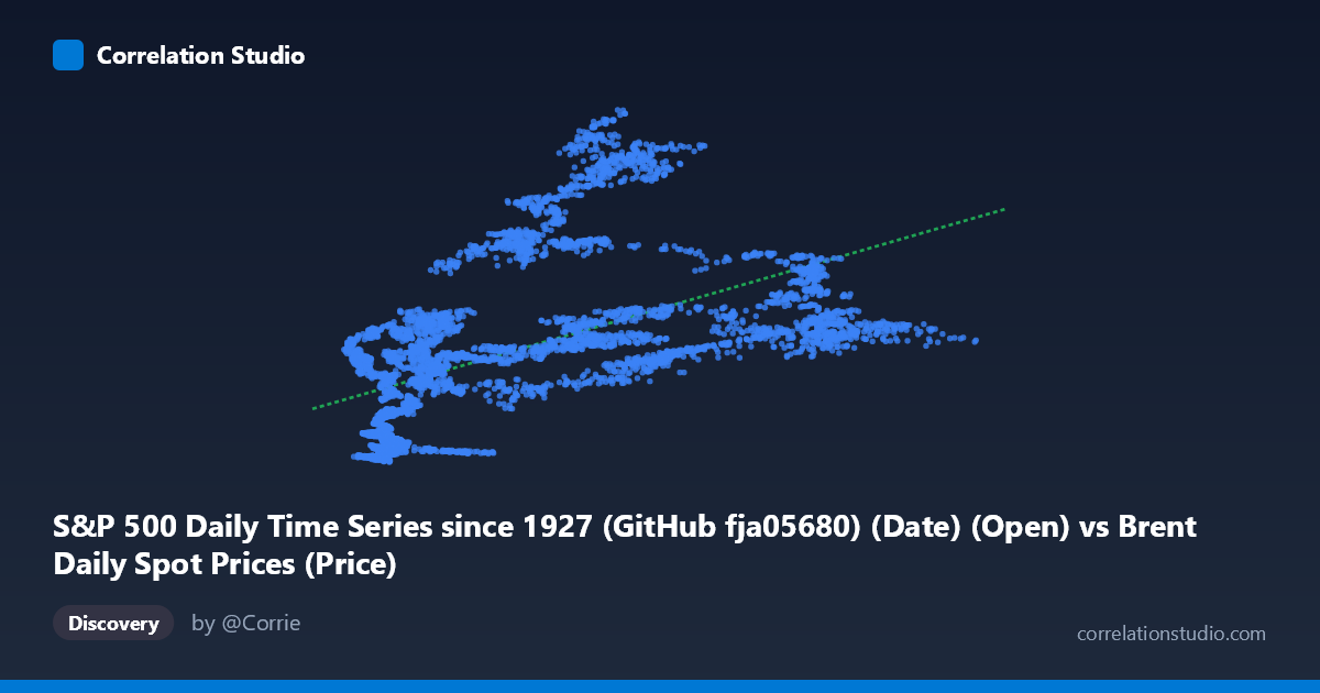
S&P 500 Daily Time Series since 1927 (GitHub fja05680) (Date) (Open) vs Brent Daily Spot Prices (Price)
- Pearson correlation (r)
- 0.5378
- Spearman correlation
- 0.6918
- p-value
- 0
- Sample size (n)
- 8140
- 95% confidence interval
- 0.5222 to 0.5531
- Granger causality
- None
- Granger optimal lag
- 1
AI analysis
Analysis: Brent Crude Oil Prices vs. S&P 500 Index
1. What the Visualization Reveals
The scatterplot displays the relationship between Brent crude oil spot prices (X-axis, in USD/barrel) and S&P 500 opening values (Y-axis), spanning over three decades from 1987 to 2019. The overall pattern shows a positive, moderately dispersed relationship — as oil prices rise, S&P 500 values tend to be higher as well. However, the cloud of data points is notably wide and heterogeneous, with considerable vertical spread at nearly every X value. This immediately signals that oil price alone is a poor standalone predictor of equity index levels. The regression line (y = 11.52x + 650.70) captures only a central tendency through substantial noise, and the scatter becomes visibly wider at higher oil price values, suggesting possible heteroscedasticity.
2. Correlation Strength, Direction, and Causality
The Pearson r of 0.5378 indicates a moderate positive correlation, but the more meaningful figure is r² = 0.2892, meaning oil prices explain only ~29% of the variance in S&P 500 levels. Roughly 71% of S&P 500 variability is driven by other factors entirely. The 95% confidence interval of [0.5222, 0.5531] is relatively narrow given the large paired sample (n = 8,140), and the p-value of essentially zero confirms the correlation is highly statistically significant — though statistical significance here reflects the massive sample size rather than practical predictive power. Critically, the Granger causality tests find no significant directional predictability in either direction (X→Y: F = 0.90, p = 0.34; Y→X: F = 0.86, p = 0.35). This is a key finding: even though the variables move together over time, neither one helps forecast the other at a one-period lag. The correlation likely reflects a shared common driver — long-run economic growth — rather than any direct causal mechanism.
3. Notable Patterns, Clusters, and Non-Linear Features
Several structural features stand out in the data. There appear to be at least two distinct clusters: a dense concentration of points at low oil prices (roughly $10–$30/barrel) paired with both low and mid-range S&P values, consistent with the 1987–2000 era, and a more dispersed cluster at higher oil values ($60–$120/barrel) with higher S&P readings, reflecting the post-2003 commodity boom and subsequent equity bull market. The note that Spearman ρ exceeds Pearson r is important — it suggests the true relationship is monotonic but non-linear, potentially logarithmic or following a curve. A few apparent outliers exist at high X values (e.g., ~$110/barrel) paired with relatively modest S&P levels (~1,288), likely corresponding to the 2008 oil price spike when equities were simultaneously collapsing — a visible contradiction of the general trend that reveals regime-dependent behavior.
4. Confounding Factors and Caveats
The most significant caveat is that both variables are time-trending upward over the sample period. The observed correlation may be largely spurious co-integration — two series rising together over decades due to inflation, monetary expansion, and global economic growth rather than any fundamental oil-equity linkage. The 2008 financial crisis likely creates a dramatic outlier regime where high oil prices coincided with crashing equities, suppressing the correlation estimate. Additionally, exchange rate effects, OPEC supply shocks, U.S. energy sector composition changes (particularly the shale revolution post-2010), and shifting correlations between oil-importing vs. oil-exporting economic dynamics all confound interpretation. The axis labels also appear swapped in the dataset metadata (oil prices labeled as S&P column and vice versa), warranting verification of data provenance before drawing firm conclusions.
5. Actionable Insights and Further Investigation
Given the non-linear signal from Spearman ρ, fitting a logarithmic or polynomial regression should be the immediate next step, likely improving explanatory power beyond the current 29%. Researchers should consider detrending both series (e.g., using log-returns or first differences) before re-computing correlation to test whether the relationship survives removal of shared secular trends — this would expose whether any genuine high-frequency co-movement exists. Regime-switching or rolling-window correlation analysis across distinct periods (pre-2000, 2000–2008, post-2008) would reveal whether the relationship is structurally stable or episodic. Finally, introducing control variables such as real GDP growth, the U.S. Dollar Index, or interest rates in a multivariate framework would help isolate whether oil price carries any incremental predictive value for equities beyond macroeconomic conditions — given the failed Granger tests, the hypothesis of independence in short-run dynamics currently holds.
X dataset: Brent Daily Spot Prices
Y dataset: S&P 500 Daily Time Series since 1927 (GitHub fja05680) (Date)
Part of experiment: Daily - Brent Daily Spot Prices vs S&P 500 Daily Time Series since 1927 (GitHub fja05680) (Date)