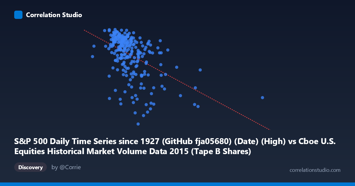
S&P 500 Daily Time Series since 1927 (GitHub fja05680) (Date) (High) vs Cboe U.S. Equities Historical Market Volume Data 2015 (Tape B Shares)
- Pearson correlation (r)
- -0.4828
- Spearman correlation
- -0.4854
- p-value
- 0
- Sample size (n)
- 252
- 95% confidence interval
- -0.5722 to -0.382
- Granger causality
- X → Y
- Granger optimal lag
- 7
AI analysis
Scatterplot Analysis: S&P 500 Daily High vs. Cboe Tape B Share Volume (2015)
Relationship Overview The scatterplot reveals a moderate negative relationship between the S&P 500 daily high price (X-axis) and Cboe Tape B share volume (Y-axis) across 252 trading days in 2015. As the S&P 500 daily high increases — ranging from approximately 44 million to 312 million in index-scaled units — Tape B share volumes tend to decline, broadly from around 2,100–2,135 down toward the 1,900–1,950 range. The linear regression equation (y = −8.496×10⁻⁷x + 2,159.73) quantifies this inverse slope, though the scatter is substantial enough that the trend is better described as a tendency than a tight rule. Visually, the bulk of observations cluster in the X range of roughly 70–130 million, where Y values span widely from ~1,920 to ~2,135, suggesting meaningful variability even within the core of the data.
Correlation Strength and Statistical Significance The Pearson correlation of r = −0.4828 indicates a moderate negative association. Critically, r² = 0.2331, meaning the S&P 500 daily high explains only about 23.3% of the variance in Tape B share volume — leaving roughly three-quarters of the variation unexplained by this linear relationship alone. The 95% confidence interval for r spans [−0.5722, −0.3820], a range that is entirely negative and meaningfully distant from zero, reinforcing that the direction of the correlation is reliable. The p-value of 4.44×10⁻¹⁶ confirms this relationship is highly statistically significant (n = 252), ruling out chance as an explanation. Importantly, the Granger causality test supports a unidirectional temporal predictive relationship: X Granger-causes Y (F = 2.159, p = 0.039) at an optimal lag of 7 trading periods (~1.5 weeks), while Y does not Granger-cause X (F = 0.685, p = 0.685). This suggests that S&P 500 price levels may have modest leading predictive power over Tape B volumes roughly one to two weeks ahead, though Granger causality establishes prediction, not true causation.
Notable Patterns, Clusters, and Outliers Several features stand out in the data. A dense central cluster forms between X ≈ 75–115 million and Y ≈ 2,050–2,135, reflecting the majority of "normal" 2015 trading days when the market was relatively elevated and volume was comparatively restrained. A distinct lower-right population appears at higher X values (150 million) paired with notably depressed Y values (~1,900–2,050), consistent with the late-August 2015 market sell-off period when equity prices dropped sharply and exchange volumes surged — though this cluster also hints at possible regime changes. Several apparent outliers exist at extreme X values (e.g., the point near X = 311 million, which falls far right of the main cluster), and a handful of low-Y observations (~1,899–1,930) at moderate X values (~111–131 million) appear to pull the regression line disproportionately. The relationship does not appear strongly non-linear, but the wide vertical scatter across the central X range suggests heteroscedasticity or omitted variables.
Confounding Factors and Caveats Several important caveats apply. First, the axis labels appear inverted relative to intuition — the X-axis is labeled as the S&P 500 "High" column from a volume dataset, and the Y-axis is labeled as "Tape B Shares" from the price dataset, suggesting a possible data join or labeling artifact that warrants verification before drawing firm conclusions. Second, both variables are time-indexed daily series in 2015, meaning autocorrelation and serial dependence are near-certain, which can inflate the effective significance of standard correlation tests. Third, market-wide shocks — particularly the August 2015 volatility spike — likely represent a distinct regime that drives much of the negative correlation signal; stripping this episode might substantially weaken or alter the relationship. Fourth, Tape B specifically covers NYSE American (AMEX) and regional exchange-listed securities, so it reflects only a subset of market activity, and its volume dynamics may respond to factors (small-cap sentiment, ETF activity) not well captured by the large-cap S&P 500 index level.
Actionable Insights and Further Investigation Practitioners should segment the analysis by market regime — separating calm periods (e.g., Q1–Q2 2015) from the August volatility episode — to determine whether the negative correlation is a persistent structural feature or primarily driven by stress periods. Given the 7-period Granger lag, a rolling window predictive model using lagged S&P 500 highs to forecast Tape B volume 7 days ahead could be worth backtesting, though the modest F-statistic (2.16) suggests limited practical predictive gain. Further investigation should incorporate VIX or realized volatility as a control variable, since fear/volatility likely co-moves with both price levels and volume in ways that could account for much of the unexplained 76.7% variance. Finally, verifying the dataset join logic — ensuring dates are properly aligned between the two source datasets — is a critical first step before any trading or research decisions are based on this correlation.
X dataset: Cboe U.S. Equities Historical Market Volume Data 2015
Y dataset: S&P 500 Daily Time Series since 1927 (GitHub fja05680) (Date)
Part of experiment: Daily - Cboe U.S. Equities Historical Market Volume Data 2015 vs S&P 500 Daily Time Series since 1927 (GitHub fja05680) (Date)