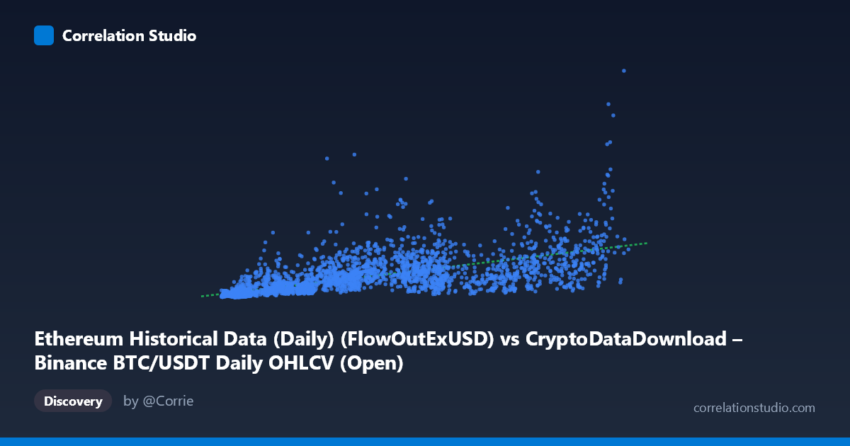
Ethereum Historical Data (Daily) (FlowOutExUSD) vs CryptoDataDownload – Binance BTC/USDT Daily OHLCV (Open)
- Pearson correlation (r)
- 0.6602
- Spearman correlation
- 0.8247
- p-value
- 0
- Sample size (n)
- 3191
- 95% confidence interval
- 0.6401 to 0.6793
- Granger causality
- Y → X
- Granger optimal lag
- 10
AI analysis
Analysis of the X–Y Relationship
1. What the Visualization Reveals
The scatterplot shows a moderate positive association between the two variables: as X (labeled "FlowOutExUSD," though the sample data ranges ~3,000–125,000, more consistent with a smaller-scale metric than raw USD flow) increases, Y (BTC/USDT Open price) tends to increase as well. However, the relationship is far from a tight linear band — there's substantial vertical scatter at every X level, particularly noticeable in the low-to-mid X range (5,000–70,000), where Y values span nearly two orders of magnitude (from ~60 million to over 1.6 billion). This spread suggests X is a contributing factor but not a dominant driver of Y.
2. Strength, Direction, and Statistical Confidence
The Pearson correlation (r = 0.660) indicates a moderate positive linear relationship, with r² = 0.436 meaning only about 44% of the variance in Y is explained by X — the majority (56%) is driven by other factors, noise, or non-linear dynamics not captured by this simple linear fit. The 95% CI [0.640, 0.679] is tight, and the p-value ≈ 0 confirms this correlation is highly unlikely to be due to chance, given the large sample (n=3,191). However, statistical significance here reflects sample size more than practical strength — a moderate r with high confidence still leaves considerable unexplained variance for forecasting purposes.
The Granger causality results are particularly noteworthy: Y Granger-causes X (F=2.013, p=0.028) at a 10-period lag, while the reverse (X→Y) is not significant (p=0.143). This implies that past values of Y (BTC price) have predictive power for future X values, but not vice versa — the causal arrow (in a predictive/temporal sense, not necessarily mechanistic) points from BTC price to the Ethereum-labeled metric. This is somewhat counterintuitive given the axis labeling and warrants a closer look at how these series were aligned/merged.
3. Notable Patterns and Outliers
Several features stand out in the sample data: - Heteroscedasticity: variance in Y increases with X in the low range, then seems to compress somewhat at higher X values — a classic sign that a log-transformation of one or both axes might linearize the relationship better. - High-Y outliers at low X: points like (11250, 667M), (14210, 703M), and (8462, 233M) show large Y values despite modest X, suggesting episodic spikes (possibly BTC bull-run periods) decoupled from the X metric. - Clustering near origin: many points cluster at X < 15,000 with Y < 150M, forming a dense low-value cluster, while a more dispersed tail extends to higher X. - The note that Spearman ρ exceeds Pearson r strongly suggests a monotonic but non-linear (likely logarithmic or power-law) relationship — common when mixing a price series (Y, BTC) with a volume/flow-type metric (X).
4. Confounding Factors and Caveats
Several caveats limit causal interpretation: - Mismatched asset labeling: the X-axis is nominally an Ethereum flow metric while Y is BTC/USDT price — both are likely driven by a common latent factor (overall crypto market sentiment, liquidity cycles, or macro conditions) rather than one directly causing the other. This shared market-wide trend (e.g., bull/bear cycles from 2017–2026) is a classic confounder. - Non-stationarity: both crypto prices and on-chain flow metrics exhibit strong trends and volatility clustering over multi-year periods; Granger causality and Pearson correlation on non-stationary series can produce spurious or inflated relationships unless differenced/detrended first. - Temporal aggregation: daily data over an 8+ year span mixes very different market regimes (2017 ICO boom, 2020-21 bull run, 2022 crash, subsequent recovery), and pooling all these regimes into one correlation obscures regime-specific dynamics.
5. Suggested Next Steps
- Re-run correlation on log-transformed variables (log(X), log(Y)) given the Spearman/Pearson discrepancy and heteroscedastic spread — this will likely substantially improve r² and yield a more interpretable power-law relationship. - Detrend/difference both series (e.g., % daily change) before Granger testing to rule out spurious causality driven by shared trends. - Segment by market regime (bull/bear/sideways) to check if the correlation strength is regime-dependent. - Verify data alignment, since the axis descriptions suggest a mismatch between the Ethereum-flow label and the BTC-price values in the samples — confirming the correct series pairing is essential before drawing further conclusions.
X dataset: CryptoDataDownload – Binance BTC/USDT Daily OHLCV
Y dataset: Ethereum Historical Data (Daily)
Part of experiment: Bitcoin - CryptoDataDownload – Binance BTC/USDT Daily OHLCV vs Ethereum Historical Data (Daily)