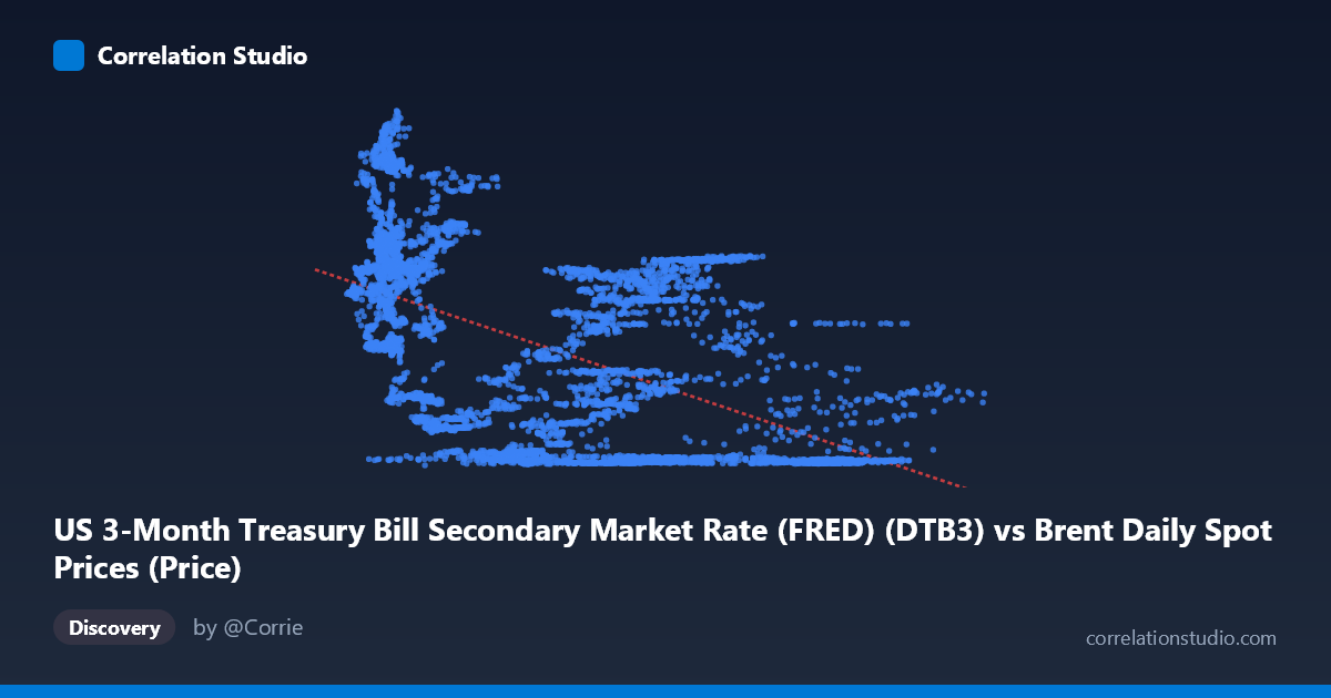
US 3-Month Treasury Bill Secondary Market Rate (FRED) (DTB3) vs Brent Daily Spot Prices (Price)
- Pearson correlation (r)
- -0.5411
- Spearman correlation
- -0.5787
- p-value
- 0
- Sample size (n)
- 9642
- 95% confidence interval
- -0.555 to -0.5268
- Granger causality
- None
- Granger optimal lag
- 1
AI analysis
Analysis: US 3-Month T-Bill Rate vs. Brent Crude Oil Spot Price
1. Overall Relationship
The scatterplot reveals a negative relationship between the US 3-Month Treasury Bill rate (X-axis) and Brent crude oil spot prices (Y-axis), summarized by the regression equation y = -0.041x + 5.099. As T-bill rates increase, oil prices tend to decrease — and conversely, low interest rate environments are associated with higher oil prices. However, the scatter is substantial and visually apparent, with data points spread widely across both axes, immediately signaling that this linear relationship captures only part of a complex story. The X-axis spans roughly 9 to 144 (USD/barrel for oil prices), while Y spans near 0 to 9% for T-bill rates, covering nearly four decades of daily observations from 1987 to 2026.
2. Correlation Strength, Direction, and Causality
The correlation coefficient of r = -0.541 indicates a moderate negative association. While statistically unambiguous — the p-value is effectively zero and the 95% confidence interval of [-0.555, -0.527] is narrow, reflecting the large sample (n = 9,642) — the practical explanatory power is modest. R² = 0.293 means that T-bill rates explain only about 29% of the variance in oil prices, leaving roughly 71% attributable to other factors. This is a meaningful but far from dominant relationship. Critically, the Granger causality tests find no significant predictive direction in either direction (X→Y: F = 1.73, p = 0.189; Y→X: F = 0.005, p = 0.944). Neither variable reliably predicts the other's future values at a one-period lag, strongly cautioning against interpreting this correlation as evidence of a directional or mechanistic link in real-time financial modeling.
3. Notable Patterns, Clusters, and Non-Linearity
Several structural features stand out in the sample points and summary statistics. There appear to be at least two distinct clusters: one dense cluster of low T-bill rates (roughly 9–30 USD/barrel oil) with widely varying oil prices (near 0 to ~9%), and another grouping at higher oil prices (70–125 USD/barrel) with near-zero T-bill rates. This bifurcation likely reflects two distinct macroeconomic regimes — the post-2008 and post-2020 zero/near-zero interest rate eras coinciding with elevated or volatile oil prices, versus earlier periods of higher rates. The relationship also appears non-linear: at very high oil prices (80 USD/barrel), T-bill rates cluster near zero, suggesting a floor effect or regime boundary rather than a smooth linear decline. A linear model may therefore be structurally misspecified for this data.
4. Confounding Factors and Caveats
Interpreting this correlation causally is fraught with confounding. Both variables are heavily influenced by shared macroeconomic drivers: recessions (e.g., 2008–09, 2020) simultaneously collapsed interest rates and disrupted oil demand; conversely, inflationary periods (early 1980s, 2021–2023) drove both rates and oil prices in complex, sometimes opposing directions. Temporal autocorrelation is almost certain in daily financial time series, which can inflate apparent correlation and undermine standard significance tests. The dataset spans 39 years across multiple monetary policy regimes (Volcker tightening, Greenspan era, zero-lower-bound periods, post-COVID tightening), making a single linear model a poor representation of any one regime. Additionally, oil prices are dollar-denominated, so USD strength — itself correlated with T-bill rates — introduces a currency confound.
5. Actionable Insights and Further Investigation
Given the regime-dependent structure of this relationship, the most productive next steps would include: (1) Regime segmentation — splitting the data into distinct monetary policy eras (e.g., pre-2008, 2008–2015 ZIRP, 2015–2019, 2020–present) and re-estimating correlations within each; (2) Non-linear modeling — fitting a piecewise regression or GAM to capture the apparent threshold behavior at high oil prices; (3) Multivariate analysis — incorporating USD index, inflation expectations (TIPS breakevens), and global demand proxies (PMI, freight rates) to isolate the independent contribution of T-bill rates; and (4) Longer Granger lags — testing causality beyond one period, as monetary policy transmission to commodity markets often operates over months, not days. The absence of Granger causality at lag-1 should not be taken as definitive; it may simply reflect that the relevant transmission horizon is longer than a single trading day.
X dataset: Brent Daily Spot Prices
Y dataset: US 3-Month Treasury Bill Secondary Market Rate (FRED)
Part of experiment: Daily - Brent Daily Spot Prices vs US 3-Month Treasury Bill Secondary Market Rate (FRED)