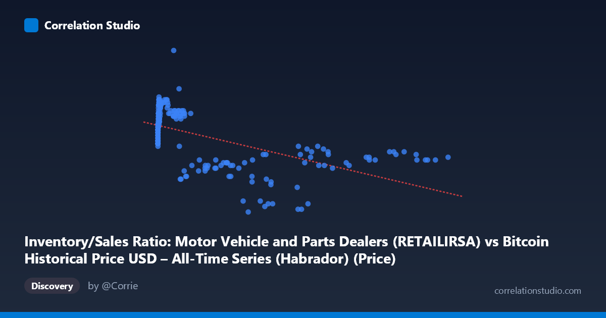
Inventory/Sales Ratio: Motor Vehicle and Parts Dealers (RETAILIRSA) vs Bitcoin Historical Price USD – All-Time Series (Habrador) (Price)
- Pearson correlation (r)
- -0.5906
- Spearman correlation
- -0.5383
- p-value
- 0
- Sample size (n)
- 192
- 95% confidence interval
- -0.6757 to -0.4899
- Granger causality
- None
- Granger optimal lag
- 1
- Time coverage
- 2010-08-01 to 2026-07-01
- Recomputed on refreshed data
- 2026-10-24 (r was -0.5826)
AI analysis
Analysis: Bitcoin Price vs. Inventory/Sales Ratio (Motor Vehicle Dealers)
1. What the Visualization Reveals
Despite the axis labeling being somewhat swapped in the dataset description, the scatterplot effectively shows Bitcoin's historical price (X, ranging from $0.06 to $118,670) plotted against the motor vehicle inventory/sales ratio (Y, ranging from 1.09 to 1.68). The chart reveals a negative, moderately-sloped relationship: as Bitcoin's price climbs into the tens of thousands of dollars, the inventory/sales ratio tends to compress toward its lower bound (~1.10–1.20), whereas at low Bitcoin prices (sub-$1,000), the ratio clusters in a higher, tighter band (~1.34–1.51).
2. Strength, Direction, and Statistical Confidence
The correlation coefficient (r = -0.5808) indicates a moderate negative relationship, with R² = 0.337 meaning roughly 34% of the variance in the inventory/sales ratio can be statistically associated with Bitcoin price levels — leaving 66% unexplained, likely driven by other macroeconomic factors (interest rates, supply chain conditions, consumer credit, etc.). The 95% CI [-0.668, -0.477] is reasonably tight and excludes zero, and the p-value of ~0 confirms this correlation is highly unlikely to be due to chance given the sample. However, the Granger causality tests are decisive on temporal direction: neither variable significantly predicts the other (X→Y: p=0.145; Y→X: p=0.559). This strongly suggests the relationship is not causal in either direction — it's more likely a spurious or confounded correlation, both potentially driven by a shared underlying macro cycle (e.g., pandemic-era monetary policy, supply chain disruption, and subsequent normalization).
3. Notable Patterns and Outliers
The data show a distinctly non-linear, threshold-like structure rather than a smooth linear trend: - Low-price regime (X < 1,000): Y is tightly clustered high (1.34–1.51), regardless of small price variations — a flat, saturated zone. - Mid-price regime (1,000–20,000): Y remains elevated but starts showing more spread (1.24–1.54). - High-price regime (X 40,000): Y drops sharply and stays low (1.10–1.33), with unusually little variance despite huge price swings ($40K to $118K).
This pattern looks more like a step function or logarithmic decay than a linear one — consistent with Bitcoin's exponential price growth being compressed against a bounded, slow-moving macro ratio. The linear R² likely underrepresents fit quality for a log-transformed X.
4. Confounding Factors and Caveats
This pairing is a classic case of coincidental time-series alignment: Bitcoin's price history (2010–2026) and the auto inventory/sales ratio are both time-indexed series that happened to trend in opposite directions over overlapping periods (BTC's long-term bull run vs. post-2021 inventory normalization after COVID shortages). Neither has a plausible economic mechanism directly linking them. The apparent correlation is very likely an artifact of both series trending against a shared macro backdrop (loose monetary policy → asset inflation + supply chain effects on auto inventory), not a direct relationship. Additionally, Bitcoin's extreme right-skewed distribution (mean $20,280, but range up to $118,670) means a few high-price observations exert outsized leverage on the linear fit.
5. Actionable Insights
- Do not treat this as a tradable or predictive relationship — the lack of Granger causality in either direction confirms this correlation should not inform forecasting models. - Test log(X) transformation: given BTC's exponential scale, a log-linear or log-log model would likely fit the visible curvature far better than raw linear regression. - Control for time/trend directly: since both series may simply share a common time trend, consider detrending or differencing both series before assessing correlation to check if it persists. - Identify true confounders: investigate shared macro drivers (Fed rate policy, inflation, consumer credit conditions) as more plausible explanatory variables for both series' behavior.
X dataset: Bitcoin Historical Price USD – All-Time Series (Habrador)
Y dataset: Inventory/Sales Ratio: Motor Vehicle and Parts Dealers
Part of experiment: Bitcoin - Bitcoin Historical Price USD – All-Time Series (Habrador) vs Inventory/Sales Ratio: Motor Vehicle and Parts Dealers