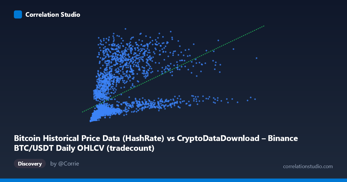
Bitcoin Historical Price Data (HashRate) vs CryptoDataDownload – Binance BTC/USDT Daily OHLCV (tradecount)
- Pearson correlation (r)
- 0.4966
- Spearman correlation
- 0.7795
- p-value
- 0
- Sample size (n)
- 3191
- 95% confidence interval
- 0.47 to 0.5223
- Granger causality
- None
- Granger optimal lag
- 10
- Time coverage
- 2017-08-17 to 2026-05-20
AI analysis
Analysis: BTC/USDT "HashRate" Column vs. Tradecount
1. Overview of the Relationship
The scatterplot shows a moderate positive association between the X variable (labeled "HashRate" but actually sourced from OHLCV price/volume fields) and Y (tradecount). Points scatter widely around the fitted regression line, with substantial spread at low X values that narrows somewhat as X increases — though even at high X values, Y ranges enormously (e.g., X≈2.39M paired with Y≈1.06B, while X≈8.7M pairs with Y≈859M, a near-reversal of expected ordering). This heteroscedastic, fan-like pattern is a hallmark of a relationship that is real but noisy, not deterministic.
2. Strength, Direction, and Statistical Confidence
The Pearson correlation (r = 0.497) indicates a moderate positive relationship, with r² = 0.247 meaning only ~25% of the variance in Y is explained by X — the remaining 75% is driven by other factors or noise. The 95% CI [0.470, 0.522] is tight given the large sample (n=3,191), and the p-value ≈ 0 confirms this correlation is highly unlikely to be due to chance. However, statistical significance ≠ practical strength: with r² this low, X alone is a weak predictor of Y.
Critically, the Granger causality tests show no significant predictive direction in either direction (X→Y: p=0.483; Y→X: p=0.922). This means neither series reliably helps forecast the other's future values based on past values, even at the optimal lag of 10 periods. Combined with the modest r², this suggests the correlation is likely driven by a shared underlying trend or common third factor (most plausibly overall Bitcoin price level/market cycle) rather than one variable mechanically driving the other.
3. Notable Patterns and Outliers
Several features stand out: - Non-monotonic clustering: Very low X values (near 0–15K) correspond to Y values spanning 4.6M to over 10M, and mid-range X values (500K–1M) produce some of the highest Y values in the sample (e.g., 795K→946M, 919K→1.09B), suggesting a possible saturation or hump-shaped curve rather than a straight line. - Compression at high X: As X exceeds ~5M, Y values cluster more tightly in the 200M–1.06B range, hinting at diminishing marginal effect — consistent with a logarithmic relationship. - The note that Spearman ρ likely exceeds Pearson r reinforces that a monotonic but non-linear (log or power-law) fit would capture more signal than the linear model, which is unsurprising given the extreme right-skew in X (mean 1.97M vastly exceeds median, per the range up to 15.36M).
4. Caveats and Confounders
- Mislabeled/ambiguous columns: The X-axis is labeled "HashRate" but its source description points to standard OHLCV fields (Open/High/Low/Close/Volume), not actual network hash rate. This metadata inconsistency should be resolved before drawing domain conclusions. - Shared time trend: Both series likely trend upward with Bitcoin's multi-year bull market (2017–2026 span), so correlation may partly reflect spurious co-trending rather than a direct mechanical link. - Scale/heteroscedasticity: Both variables have huge dynamic ranges (X: 2K–15.4M; Y: 4M–1.3B) with high stdev relative to mean, meaning a few large-scale periods (e.g., bull-market peaks) could disproportionately drive the linear fit. - Non-stationarity: Financial/crypto time series are typically non-stationary; Granger causality tests on raw (non-differenced) data can be unreliable — the "no causality" finding may partly reflect this rather than true independence.
5. Recommendations for Further Investigation
1. Verify column semantics — confirm whether X truly represents hash rate, volume, or price, as this changes the entire economic interpretation. 2. Re-run correlation on log-transformed variables or fit a log/power model, given the skewed distributions and the Spearman/Pearson divergence. 3. De-trend or difference both series (e.g., % daily change) before re-testing Granger causality, since raw price/volume-linked series are usually non-stationary and can mask or fabricate causal signals. 4. Segment by market regime (bull vs. bear phases) to check if the r²=0.25 relationship is stable or concentrated in specific periods. 5. Treat this as a descriptive, not predictive relationship — given the null Granger result, avoid using X to forecast Y (or vice versa) in trading or modeling contexts without further evidence of a mechanistic link.
X dataset: CryptoDataDownload – Binance BTC/USDT Daily OHLCV
Y dataset: Bitcoin Historical Price Data
Part of experiment: Bitcoin - CryptoDataDownload – Binance BTC/USDT Daily OHLCV vs Bitcoin Historical Price Data