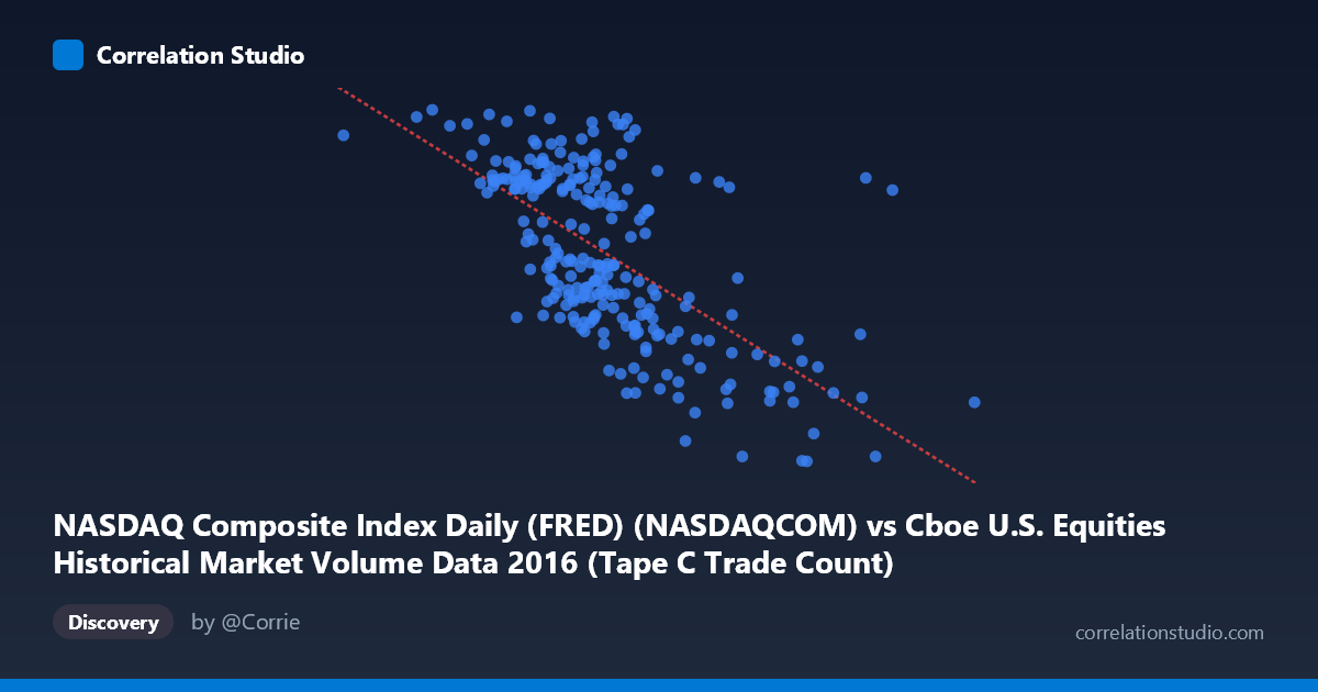
NASDAQ Composite Index Daily (FRED) (NASDAQCOM) vs Cboe U.S. Equities Historical Market Volume Data 2016 (Tape C Trade Count)
- Pearson correlation (r)
- -0.6412
- Spearman correlation
- -0.6383
- p-value
- 0
- Sample size (n)
- 252
- 95% confidence interval
- -0.7086 to -0.5622
- Granger causality
- None
- Granger optimal lag
- 10
AI analysis
Analysis: NASDAQ Composite Index vs. Cboe Tape C Trade Count (2016)
Relationship Overview The scatterplot reveals a negative relationship between the NASDAQ Composite Index level and Cboe Tape C Trade Count across 2016. As the NASDAQ index climbed to higher values, the number of trades on Tape C venues tended to decline. This is a somewhat counterintuitive finding at first glance — rising equity prices coinciding with fewer trades — but it aligns with well-documented market microstructure dynamics where bull market complacency and reduced volatility suppress trading activity. The linear regression equation (y = −0.0013x + 5,916.86) quantifies this inverse slope, with trade counts falling by roughly 1.3 units for every 1,000-point increase in the index.
Correlation Strength and Statistical Framing The Pearson correlation of r = −0.6412 indicates a moderate-to-strong negative association, and the R² of 0.4112 means that approximately 41% of the variance in Tape C trade counts is explained by the NASDAQ index level — a meaningful but incomplete explanation, leaving 59% attributable to other factors. The 95% confidence interval of [−0.7086, −0.5622] is notably tight and does not cross zero, and the p-value of effectively 0 across n = 252 paired observations drawn from a population of N = 3,622 provides very strong evidence that this correlation is not a sampling artifact. However, the Granger causality results are unambiguous in their null finding: neither direction (X→Y: F = 0.163, p = 0.998; Y→X: F = 0.479, p = 0.903) approaches significance at any conventional threshold, even with an optimal lag of 10 periods. This means that knowing today's NASDAQ level does not help predict tomorrow's trade count, and vice versa — the correlation is likely driven by a shared underlying temporal trend rather than any direct predictive mechanism between the two series.
Notable Patterns, Clusters, and Outliers Several structural features stand out in the data. The bulk of observations cluster in the X range of roughly 580,000–800,000 with Y values between 4,700 and 5,400, forming a dense central cloud with a visible downward tilt. There are notable high-X outliers in the 900,000–1,050,000+ range (e.g., points near 990,202 and 1,023,027) that pair with conspicuously low trade counts (~4,450–4,510), pulling the regression line and likely inflating the correlation's apparent strength. Conversely, some lower-X points (e.g., ~504,690 and ~519,410) show high trade counts near the top of the Y range (~5,230–5,470), consistent with elevated volatility and volume during early 2016 market stress. There is also visible vertical spread across the central cluster, suggesting heteroscedasticity — variance in trade counts appears larger at moderate index levels than at extremes.
Confounding Factors and Caveats This correlation almost certainly reflects temporal co-movement rather than a causal mechanism. Both variables are time-indexed through 2016: the NASDAQ trended upward over the year while market volumes on certain venues trended downward, potentially due to structural shifts in exchange competition, maker-taker fee changes, or migration of volume to alternative venues. The NASDAQ index is a price/valuation measure while Tape C trade count is a microstructure activity measure — they operate on fundamentally different scales and mechanisms. Additionally, the lack of Granger causality strongly suggests a spurious correlation driven by a common third factor (e.g., the passage of time, VIX/volatility regime, or secular volume trends). The sample (n = 252) represents only one calendar year, limiting generalizability, and the presence of high-leverage outliers at extreme X values warrants scrutiny.
Actionable Insights and Further Investigation Given the strong correlation but absent Granger causality, the most productive next step would be to partial out the time trend from both series (e.g., via first-differencing or detrending) and retest the correlation — if r collapses near zero, the relationship is likely spurious. It would also be valuable to incorporate VIX or realized volatility as a covariate, since volatility is a well-established driver of trading volume and may mediate or confound this relationship entirely. Examining other Tape designations (Tape A and B) under the same framework would clarify whether this is a Tape C–specific phenomenon or a broader market effect. Finally, extending the analysis across multiple years (the underlying dataset spans 1971–present for NASDAQ) could reveal whether this negative relationship is stable or unique to 2016's particular market conditions.
X dataset: Cboe U.S. Equities Historical Market Volume Data 2016
Y dataset: NASDAQ Composite Index Daily (FRED)
Part of experiment: Daily - Cboe U.S. Equities Historical Market Volume Data 2016 vs NASDAQ Composite Index Daily (FRED)