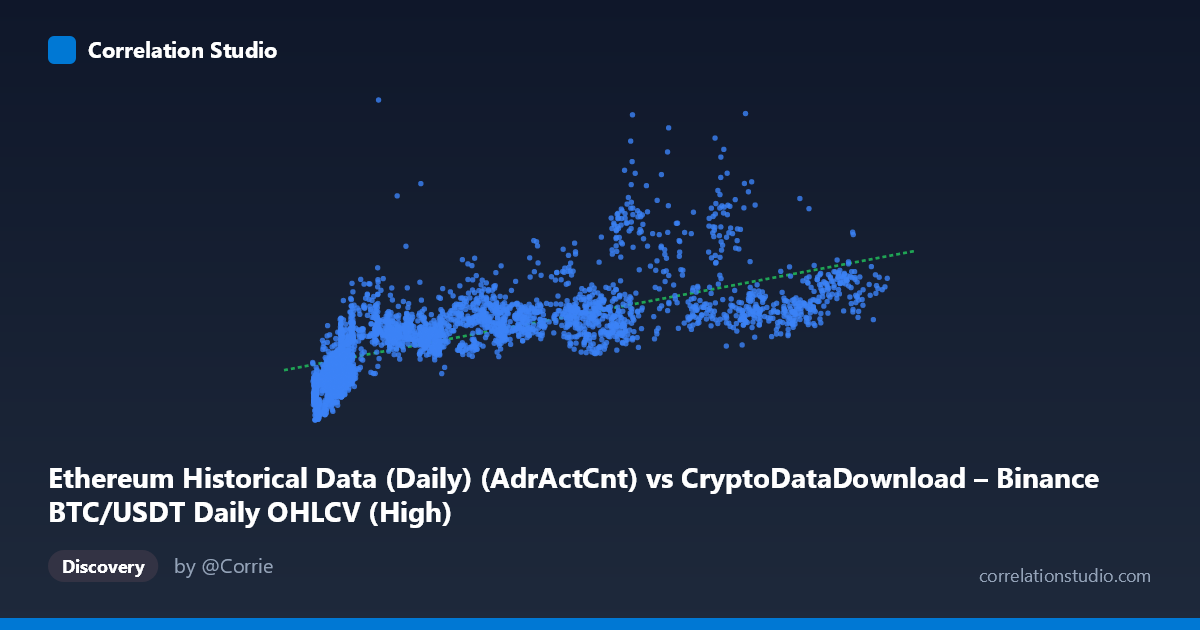
Ethereum Historical Data (Daily) (AdrActCnt) vs CryptoDataDownload – Binance BTC/USDT Daily OHLCV (High)
- Pearson correlation (r)
- 0.6972
- Spearman correlation
- 0.8297
- p-value
- 0
- Sample size (n)
- 3191
- 95% confidence interval
- 0.6789 to 0.7146
- Granger causality
- None
- Granger optimal lag
- 10
AI analysis
Analysis: Ethereum Active Address Count vs. BTC/USDT Daily High Price
(Note: the axis labels appear mismatched with the described datasets — X is labeled "AdrActCnt" but the source is listed as BTC/USDT OHLCV, while Y is labeled BTC High but sourced from Ethereum metrics. The analysis below treats X and Y as given numerically, but this labeling inconsistency should be resolved before drawing final conclusions.)
1. Overview of the Relationship
The scatterplot shows a moderate-to-strong positive association between X and Y: as X increases from its minimum (~3,277) toward its maximum (~126,200), Y generally rises from the low hundred-thousands toward 1.5 million. The relationship is not perfectly linear — points fan out and thicken at low-to-mid X values, then thin out at high X, suggesting a concave or logarithmic shape rather than a straight line.
2. Strength, Direction, and Statistical Confidence
The Pearson correlation of r = 0.697 indicates a moderately strong positive linear relationship, with r² = 0.486 meaning roughly 49% of the variance in Y is explained by X — leaving over half of Y's variability attributable to other factors, noise, or nonlinear dynamics not captured by the linear model. The 95% CI [0.679, 0.715] is tight given the large sample (n=3,191), and the p-value of ~0 confirms this correlation is highly statistically significant — it is very unlikely to be a chance artifact. However, statistical significance here should not be conflated with strong predictive power; r² near 0.5 leaves substantial unexplained variance. Critically, the Granger causality tests show no significant predictive direction in either direction (X→Y: p=0.74; Y→X: p=0.67) at the optimal lag of 10 periods. This means neither series reliably precedes or forecasts changes in the other over time — the contemporaneous correlation likely reflects a shared external driver (e.g., overall market cycle, adoption trends, or macro sentiment) rather than one variable causing the other.
3. Notable Patterns and Non-linearity
The data shows clear heteroscedasticity: variance in Y increases substantially as X grows, producing a fan/cone shape. At low X (roughly 3,000–15,000), Y values cluster tightly between 150,000–500,000, but at mid-range X (60,000–90,000), Y spreads widely from ~500,000 to over 1,500,000 — indicating other factors dominate Y's behavior in this range. Several notable outliers exist: points like (68,653, 999,185) and (90,741, 860,816) sit well above the general trend, while (84,300, 520,203) sits below it — suggesting episodic decoupling, possibly tied to distinct market regimes or events. The note that Spearman ρ exceeds Pearson r reinforces that a monotonic but curved relationship (log or power-law) likely fits better than the straight-line OLS model, consistent with diminishing returns as X grows.
4. Confounding Factors and Caveats
Both variables are time-series drawn from cryptocurrency markets over an overlapping 2017–2026 window, making them prone to spurious correlation via shared trends — both crypto prices and network activity metrics tend to rise and fall together during bull/bear cycles, independent of direct causal linkage. Autocorrelation within each series (trending data) can inflate Pearson r without indicating a genuine bivariate relationship. The lack of Granger causality supports this concern: the correlation may be driven by a common latent factor (overall market cycle, speculative sentiment, macro liquidity) rather than any direct mechanistic link between the two metrics.
5. Suggested Next Steps
1. Verify axis/variable labeling — the mismatch between axis titles and dataset descriptions should be resolved before further modeling. 2. Fit non-linear models (log-log, power, or polynomial regression) given the Spearman/Pearson divergence and visible fan-shaped variance. 3. Detrend or difference both series before correlating, to test whether the relationship holds beyond shared trend/cycle effects (spurious correlation check). 4. Segment by market regime (bull vs. bear periods) to see if the relationship strengthens or breaks down in specific phases — this could explain the widening spread at higher X. 5. Investigate outlier periods (e.g., the 999,185 and 860,816 Y-value points) for specific market events that may explain temporary decoupling.
X dataset: CryptoDataDownload – Binance BTC/USDT Daily OHLCV
Y dataset: Ethereum Historical Data (Daily)
Part of experiment: Bitcoin - CryptoDataDownload – Binance BTC/USDT Daily OHLCV vs Ethereum Historical Data (Daily)