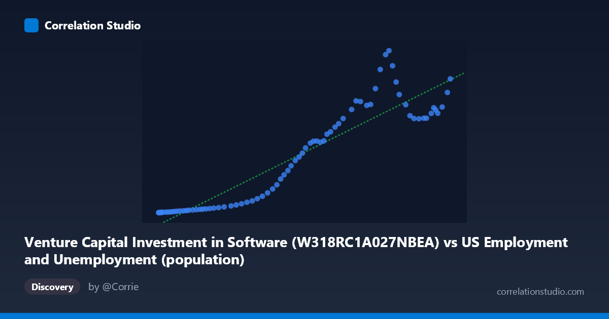
Venture Capital Investment in Software (W318RC1A027NBEA) vs US Employment and Unemployment (population)
- Pearson correlation (r)
- 0.9281
- Spearman correlation
- 0.9574
- p-value
- 0
- Sample size (n)
- 79
- 95% confidence interval
- 0.8895 to 0.9535
- Granger causality
- None
- Granger optimal lag
- 10
- Time coverage
- 1946-01-01 to 2024-01-01
AI analysis
Analysis of Venture Capital Investment in Software vs. US Population (1946–2024)
1. What the Visualization Reveals
The scatterplot reveals a strong positive relationship between Venture Capital (VC) investment in software and US population over the annual time series spanning 1946 to 2024. As VC investment in software increases, the US population rises in tandem, tracing a broadly upward trajectory across the full range of observations. The data points cluster tightly around the fitted regression line (y = 0.00251614x − 293.319), with relatively modest scatter, suggesting the two variables move together in a consistent and systematic way across nearly eight decades of data.
2. Strength, Direction, and Statistical Framing
The Pearson correlation coefficient of r = 0.928 indicates a very strong positive association, and the R² of 0.861 means that approximately 86.1% of the variance in US population is statistically explained by variation in VC software investment within this linear model. The 95% confidence interval for r ([0.890, 0.954]) is narrow and entirely positive, reflecting high precision in the estimate given the sample size of n = 79. The p-value of effectively zero confirms this is extremely unlikely to be a chance result. However, the Granger causality tests tell a critically important story: neither direction (X→Y nor Y→X) reaches significance (F = 0.41, p = 0.93 and F = 0.65, p = 0.76, respectively, at optimal lag 10). This means that knowing past values of VC investment does not help predict future population, and vice versa — strongly implying the correlation, however numerically impressive, does not reflect a meaningful predictive or causal mechanism between these two specific variables.
3. Notable Patterns, Clusters, and Outliers
The data points at the lower-left of the chart (X ≈ 103,000–130,000; Y ≈ 0.85–12) form a dense cluster corresponding to the earlier decades of the time series, when both VC investment in software was minimal and the population was lower. The upper-right region shows considerably more dispersion, with several notable points standing out: (231,867; 455.02), (233,788; 466.42), and (235,801; 422.88) appear as potential high-leverage outliers sitting above the general trend, suggesting episodes where population values were elevated relative to what the linear model predicts. Conversely, points like (250,801; 270.67) and (253,538; 272.29) fall noticeably below the trend line at high X values, hinting at possible non-linearity or regime changes in the upper range — perhaps reflecting periods where VC investment surged without proportional population growth. A mild S-curve or segmented pattern may be present and would warrant testing a polynomial or piecewise fit.
4. Confounding Factors and Caveats
The most fundamental caveat here is spurious correlation driven by shared secular time trends. Both US population and VC investment in software are strongly trended upward over time — population grows through demographics, and VC investment has grown exponentially with the technology sector's rise. Any two upward-trending time series measured over the same period will tend to correlate strongly regardless of any true relationship. The Granger causality failure confirms this suspicion. Additional confounders include: macroeconomic growth (GDP), inflation affecting nominal VC figures, post-WWII baby boom dynamics, and the structural transformation of the US economy toward technology. The dataset label metadata also appears potentially transposed (the X-axis dataset is labeled "US Employment and Unemployment" while the Y-axis is labeled "Venture Capital Investment in Software"), which introduces ambiguity about what precisely is being measured on each axis and warrants verification before drawing any substantive conclusions.
5. Actionable Insights and Further Investigation
Given the strong correlation but absent Granger causality, the priority next step should be detrending both series (e.g., first-differencing or HP filtering) and re-examining whether any relationship persists after removing the shared time trend — this would reveal whether the correlation is genuinely informative or purely an artifact of parallel growth. Researchers should also test for cointegration (e.g., Engle-Granger or Johansen tests), since two non-stationary series can have a meaningful long-run equilibrium even without short-run Granger causality. Investigating the outlier years (approximately 2000–2003 dot-com era and 2021–2022 VC boom periods) as structural breaks could improve model fit. Finally, clarifying the axis label discrepancy and confirming the exact variables being plotted is essential — pairing VC investment with tech-sector employment or productivity, rather than total population, would likely yield a more theoretically grounded and interpretable analysis.
X dataset: US Employment and Unemployment
Y dataset: Venture Capital Investment in Software
Part of experiment: Yearly - US Employment and Unemployment vs Venture Capital Investment in Software